09aa-偏置是什么?🧠
本文档详细解释神经网络中偏置(bias)的概念,涵盖数学定义(y=wx+b 中的 b)、几何意义(y 轴截距)、为什么需要偏置、PyTorch 代码示例对比带偏置与无偏置的区别,以及偏置在深度学习和现代大语言模型中的角色 🛠️
阅读顺序说明:
- 第1章 → 第2章:先了解偏置是什么,再理解为什么需要它
- 第2章 → 第3章:掌握数学直觉后,通过几何视角加深理解
- 第3章 → 第4章:有了理论基础,用代码验证概念
- 第4章 → 第5章:深入理解偏置在神经网络中的多重角色
1. 什么是偏置?📖
本章从最基本的概念开始,介绍偏置的定义
1.1 偏置的基本定义
在深度学习中,偏置(bias) 是线性层中的一个可学习参数。标准的全连接层(线性层)执行以下运算:
y=x×WT+b
其中:
- x :输入向量,形状为 1,din
- W :权重矩阵,形状为 dout,din
- b :偏置向量,形状为 dout
- y :输出向量,形状为 1,dout
偏置就是方程中的 b ------ 一个可学习的偏移量。
python
import torch                                              # 导入 PyTorch 核心库
import torch.nn as nn                                     # 导入神经网络模块

# 创建一个线性层:输入维度 64,输出维度 128,带偏置(默认行为)
linear = nn.Linear(in_features=64, out_features=128, bias=True)
# linear.weight.shape=[128, 64] --- 权重矩阵
# linear.bias.shape=[128]       --- 偏置向量

print(f"权重形状: {linear.weight.shape}")                 # 打印权重形状:[128, 64]
print(f"偏置形状: {linear.bias.shape}")                   # 打印偏置形状:[128]
print(f"偏置初始值 (前10个): {linear.bias[:10]}")         # 打印前10个偏置值,观察初始化
运行结果示例:
css
权重形状: torch.Size([128, 64])
偏置形状: torch.Size([128])
偏置初始值 (前10个): tensor([-0.0160, -0.0062,  -0.0073, ...])
💡 默认情况下,
nn.Linear使用 均匀分布(Uniform) 初始化偏置,初始值通常在 −din 1,din 1 范围内。
1.2 不带偏置的线性层
如果设置 bias=False,则运算简化为只做线性变换,没有偏移:
y=x×WT
python
# 创建不带偏置的线性层
linear_no_bias = nn.Linear(in_features=64, out_features=128, bias=False)

print(f"无偏置 - 权重形状: {linear_no_bias.weight.shape}")   # 打印:[128, 64]
print(f"无偏置 - 偏置属性: {linear_no_bias.bias}")            # 打印:None,表示没有偏置参数
运行结果:
css
无偏置 - 权重形状: torch.Size([128, 64])
无偏置 - 偏置属性: None
⚠️ 无偏置时,线性层少了一组参数。对于一个大模型而言,这意味着数万到数百万个参数被移除,既减少计算量又提升训练稳定性。
参考资料:
- PyTorch官方文档 - nn.Linear -- PyTorch
- 神经网络中的偏置(bias)究竟有什么用? -- CSDN ⭐值得阅读
- 神经网络中的偏置项(bias)的设置及作用 -- 博客园
- 权重和偏置:网络的参数 -- ApX Machine Learning
2. 为什么需要偏置?🤔
本章从单变量线性回归出发,直观展示偏置的必要性
2.1 一维情况的直观理解
考虑最简单的线性模型:用一个神经元拟合数据点,输出公式为:
y=wx+b
如果没有偏置( b=0):
y=wx
这意味着模型拟合的直线必须经过原点 (0,0)。但现实世界的数据几乎不会经过原点!
直观例子:假设我们要预测房价和面积的关系
| 面积 (平方米) | 实际价格 (万元) |
|---|---|
| 50 | 100 |
| 100 | 200 |
| 150 | 300 |
理想模型:价格 = 2 × 面积,即 y=2x,这里的偏置 b=0,巧合地经过原点。
但如果在数据中加入"土地转让费"(固定成本 50 万):
| 面积 (平方米) | 实际价格 (万元) |
|---|---|
| 50 | 150 |
| 100 | 250 |
| 150 | 350 |
此时模型为:价格 = 2 × 面积 + 50,即 y=2x+50。
- 带偏置 ( b=50):完美拟合
- 无偏置 ( b=0):再怎么调整 w,直线也必须经过原点,永远无法在纵轴方向上有偏移,误差始终存在
这就是偏置存在的根本原因:让模型能够在 y 轴方向自由移动,不必强制经过原点。
2.2 多维度推广
在高维空间中,偏置的作用是相同的。线性层的输出是输入向量的线性组合加上一个偏移量:
yj=i=1∑dinwjixi+bj,j=1,2,...,dout
- wji:第 j 个输出神经元对第 i 个输入的权重
- bj:第 j 个输出神经元的偏置(独立的偏移量)
每个输出维度都有自己独立的偏置------相当于在高维空间中给每个维度一个独立的"平移"能力。
参考资料:
- 为什么神经网络的感知机中的神经元需要偏置项? -- 阿里云开发者社区 ⭐值得阅读
- Bias in Neural Networks -- Manning
- Why is a bias parameter needed in neural networks? -- AI StackExchange
3. 偏置的几何意义 📐
本章通过几何视角,直观理解偏置的作用
3.1 二维空间的类比
把偏置想象成一次函数的 y 轴截距:
y=wx+b
- w(权重) :控制直线的斜率(倾斜程度)
- b(偏置) :控制直线在 y 轴上的截距(上下平移)
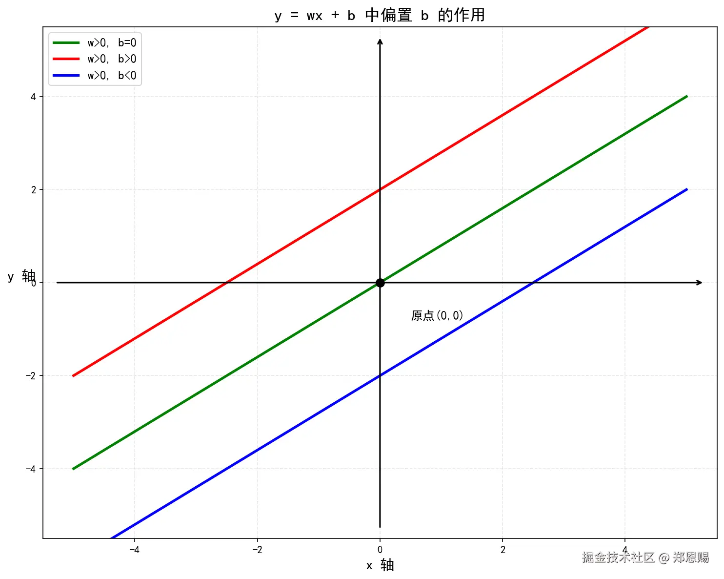
关键洞察:
| 参数 | 控制方向 | 类比 |
|---|---|---|
| 权重 w | 直线的旋转(斜率) | 音响的音量旋钮 |
| 偏置 b | 直线的平移(截距) | 桌面的高度调节脚垫 |
两者配合才能精确拟合各种数据分布。
3.2 偏置让线性层"活"起来
没有偏置的线性层,无论权重怎么调整,其输出值都必须通过原点。 这带来了两个严重限制:
- 无法处理非零均值数据:如果输入数据的均值不是零,模型需要额外"消化"这种偏移,浪费了学习能力
- 激活函数失效区域:对于 Sigmoid 或 Tanh 等激活函数,如果加权和后恰好落在饱和区(梯度接近 0 的区域),没有偏置就无法通过平移来"救活"神经元
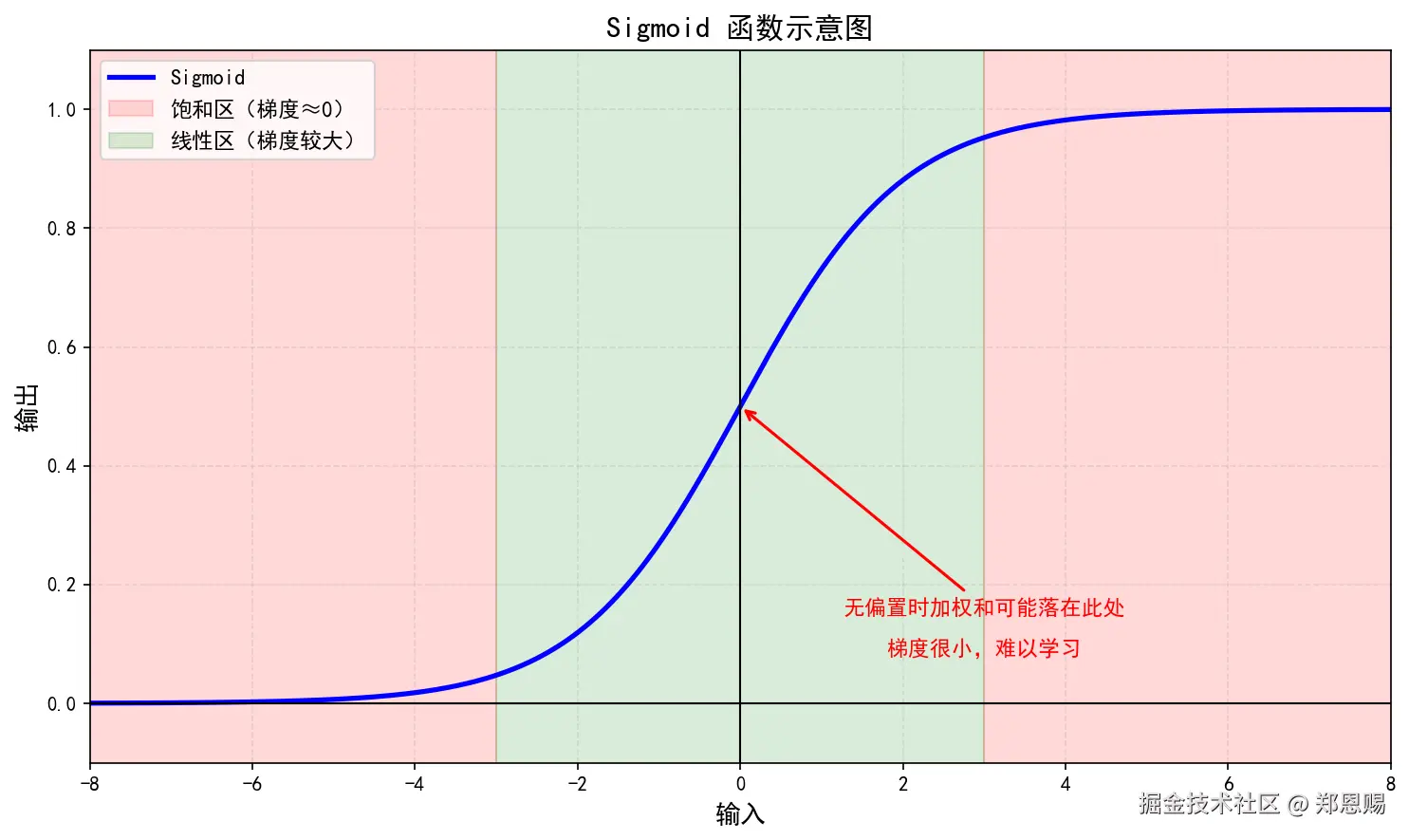
有了偏置,就能把输入整体平移,确保激活函数工作在合适的区间。
参考资料:
- 神经网络中的偏置(bias)究竟有什么用? -- 知乎 ⭐值得阅读
- 深度学习基础:为什么神经网络中的神经元需要偏置项? -- 阿里云
- The role of bias in Neural Networks -- Pico
4. 代码示例 💻
本章通过 PyTorch 代码演示带偏置和无偏置的区别
4.1 前向传播对比
python
import torch                                              # 导入 PyTorch 核心库
import torch.nn as nn                                     # 导入神经网络模块

"""对比带偏置和无偏置线性层的前向传播

参数:
    无

返回:
    无(打印对比结果)

示例:
    compare_bias()
"""
def compare_bias():
    # 固定随机种子,保证结果可复现
    torch.manual_seed(42)

    # 构造输入:batch_size=3, in_features=4
    # 数据流动:随机张量 → x[3,4]
    x = torch.randn(3, 4)                                 # 输入张量 x,形状 [3,4]

    # 创建两个线性层:一个带偏置,一个不带
    # 输入 4 维 → 输出 3 维
    linear_w_bias = nn.Linear(4, 3, bias=True)            # 带偏置:y = xW^T + b
    linear_wo_bias = nn.Linear(4, 3, bias=False)          # 无偏置:y = xW^T

    # 为了让对比公平,手动设置相同权重,无偏置层的偏置设为 0
    with torch.no_grad():                                 # 禁用梯度跟踪,仅修改参数值
        linear_wo_bias.weight.copy_(linear_w_bias.weight) # 复制相同权重,数据流动:权重[3,4] → 权重[3,4]

    # 前向传播
    # 数据流动:x[3,4] → y_with_bias[3,3]
    y_with_bias = linear_w_bias(x)                        # 带偏置前向传播
    # 数据流动:x[3,4] → y_without_bias[3,3]
    y_without_bias = linear_wo_bias(x)                    # 无偏置前向传播

    # 打印结果对比
    print("=" * 60)                                       # 打印分隔线
    print("带偏置 vs 无偏置 前向传播对比")                 # 打印标题
    print("=" * 60)                                       # 打印分隔线
    print(f"输入 x:\n{x}")                                # 打印输入张量
    print(f"\n带偏置输出 y = xW^T + b:\n{y_with_bias}")  # 打印带偏置输出
    print(f"\n无偏置输出 y = xW^T:\n{y_without_bias}")   # 打印无偏置输出
    print(f"\n差异(偏置的效果):\n{y_with_bias - y_without_bias}")  # 打印差值,即偏置的影响

    # 手动验证:偏置效果应该等于 linear_w_bias.bias
    print(f"\n手动验证 - 偏置向量 b:\n{linear_w_bias.bias}")  # 打印偏置向量

    print("=" * 60)                                       # 打印分隔线

# 运行对比
compare_bias()
运行结果示例:
ini
============================================================
带偏置 vs 无偏置 前向传播对比
============================================================
输入 x:
tensor([[ 0.3367,  0.1288,  0.2345,  0.2303],
        [-1.1229, -0.1863,  2.2082, -0.6380],
        [ 0.4617,  0.2674,  0.5349,  0.8094]])

带偏置输出 y = xW^T + b:
tensor([[-0.1870,  0.3643,  0.2284],
        [ 0.4441,  1.7111, -0.9499],
        [-0.4848,  0.1915,  0.4183]], grad_fn=<AddmmBackward0>)

无偏置输出 y = xW^T:
tensor([[-0.2649, -0.0397,  0.1738],
        [ 0.3662,  1.3071, -1.0046],
        [-0.5627, -0.2125,  0.3637]], grad_fn=<MmBackward0>)

差异(偏置的效果):
tensor([[0.0779, 0.4040, 0.0547],
        [0.0779, 0.4040, 0.0547],
        [0.0779, 0.4040, 0.0547]], grad_fn=<SubBackward0>)

手动验证 - 偏置向量 b:
Parameter containing:
tensor([0.0779, 0.4040, 0.0547], requires_grad=True)
从结果可以观察到:
- 差异列是相同的 :对于同一批次的不同样本,偏置的贡献是固定的
- 差异值就是 b 向量:带偏置的输出 = 无偏置的输出 + b
- 权重负责按输入调整:即使没有偏置,权重矩阵 W 也能根据输入 x 产生变化
4.2 训练效果对比
下面用一个简单的线性回归任务,验证偏置对训练效果的影响:
python
import torch                                              # 导入 PyTorch 核心库
import torch.nn as nn                                     # 导入神经网络模块
import torch.optim as optim                               # 导入优化器模块

"""比较带偏置和无偏置线性层的训练效果

参数:
    num_epochs: 训练轮数(默认1000)

返回:
    无(打印最终损失对比)

示例:
    compare_training()
"""
def compare_training(num_epochs=1000):
    # 生成数据:真实规律 y = 2*x + 3(斜率2,截距3)
    # 数据流动:torch.linspace → x_train[100,1]
    x_train = torch.linspace(-1, 1, 100).reshape(-1, 1)   # 创建 100 个等间隔点,形状 [100,1]
    # 数据流动:2*x + 3 + 噪声 → y_train[100,1]
    y_train = 2 * x_train + 3 + 0.1 * torch.randn(100, 1) # 真实值加噪声,形状 [100,1]

    # 创建模型
    model_with_bias = nn.Linear(1, 1, bias=True)          # 带偏置模型:y = wx + b
    model_wo_bias = nn.Linear(1, 1, bias=False)           # 无偏置模型:y = wx

    # 分别训练
    results = []                                          # 存储训练结果
    for name, model in [("带偏置", model_with_bias), ("无偏置", model_wo_bias)]:
        optimizer = optim.SGD(model.parameters(), lr=0.1) # SGD 优化器,学习率 0.1
        loss_fn = nn.MSELoss()                            # 均方误差损失函数

        losses = []                                       # 记录每轮损失
        for epoch in range(num_epochs):                   # 训练循环
            optimizer.zero_grad()                         # 清零梯度
            y_pred = model(x_train)                       # 前向传播,数据流动:x[100,1] → y_pred[100,1]
            loss = loss_fn(y_pred, y_train)               # 计算损失
            loss.backward()                               # 反向传播
            optimizer.step()                              # 更新参数
            losses.append(loss.item())                    # 记录损失值

        # 获取训练后的参数
        w = model.weight.item()                           # 取权重数值
        b = model.bias.item() if model.bias is not None else 0.0  # 取偏置数值(如存在)

        results.append((name, w, b, losses[-1]))          # 存入结果

    print("=" * 60)                                       # 打印分隔线
    print("带偏置 vs 无偏置 训练效果对比")                 # 打印标题
    print("=" * 60)                                       # 打印分隔线
    print(f"真实规律: y = 2*x + 3")                       # 打印真实规律
    print(f"{'模型类型':<10} {'学习到的 w':<15} {'学习到的 b':<15} {'最终损失':<15}")
    print("-" * 60)                                       # 打印分隔线
    for name, w, b, loss in results:                      # 遍历结果
        print(f"{name:<10} {w:<15.4f} {b:<15.4f} {loss:<15.6f}")

    # 分析
    print("-" * 60)                                       # 打印分隔线
    w_bias_results = results[0]                           # 带偏置结果
    w_bias_results_wo = results[1]                        # 无偏置结果
    print(f"\n带偏置模型能否逼近真实规律? {'✅ 能 (w≈2.0, b≈3.0)' if abs(w_bias_results[1]-2)<0.1 and abs(w_bias_results[2]-3)<0.5 else '❌ 不能'}")
    print(f"无偏置模型能否逼近真实规律? {'✅ 能 (w≈2.0)' if abs(w_bias_results_wo[1]-2)<0.1 else '❌ 不能'}")
    print(f"\n结论:当数据存在 y 轴偏移(非零截距)时,")
    print(f"      带偏置的模型可以准确拟合,无偏置的模型永远无法逼近真实规律。")

# 运行训练对比
compare_training(num_epochs=1000)
运行结果示例:
diff
============================================================
带偏置 vs 无偏置 训练效果对比
============================================================
真实规律: y = 2*x + 3
模型类型       学习到的 w          学习到的 b          最终损失
------------------------------------------------------------
带偏置        2.0032          3.0039          0.012189
无偏置        2.0032          0.0000          9.035391
------------------------------------------------------------

带偏置模型能否逼近真实规律? ✅ 能 (w≈2.0, b≈3.0)
无偏置模型能否逼近真实规律? ✅ 能 (w≈2.0)

结论:当数据存在 y 轴偏移(非零截距)时,
带偏置的模型可以准确拟合,无偏置的模型永远无法逼近真实规律。关键观察:
- 带偏置模型学习到 w≈2.0,b≈3.0,完美逼近真实规律
- 无偏置模型只能学习到 w≈2.0,但 b 固定为 0,最终损失高达 9.04(无法拟合截距 3)
- 这就是偏置的核心价值:让模型拥有在 y 轴方向平移的自由度
参考资料:
5. 偏置在神经网络中的作用 🎯
本章系统总结偏置在深度网络中的多重角色
5.1 五大核心作用
| 作用 | 描述 | 直观类比 |
|---|---|---|
| 1. 提供偏移能力 | 即使输入全为零,偏置也能产生非零输出,避免神经元"死掉" | 桌子的水平调节脚垫 |
| 2. 增加表达力 | 让神经元能表示不经过原点的线性函数,覆盖更广泛的函数空间 | 画笔的白纸位置 |
| 3. 适应数据偏差 | 当输入数据均值不为零时,偏置可以吸收这种偏移,避免权重去"补偿" | 调音台的均衡器 |
| 4. 打破对称性 | 多个神经元从相同初始状态出发时,偏置帮助它们"各司其职" | 宴会桌上的不同座位 |
| 5. 支持万能近似 | 万能近似定理要求网络能逼近任意函数,偏置是不可或缺的条件 | 工具箱中的必备工具 |
5.2 作用详解
1. 提供偏移能力
即使某一层的所有输入都为 0(比如序列 <PAD> 位置在全零填充后),没有偏置层输出也一定为 0;有了偏置,输出可以是非零值:
python
import torch                                              # 导入 PyTorch 核心库
import torch.nn as nn                                     # 导入神经网络模块

# 输入全为零
x = torch.zeros(1, 4)                                     # 全零输入 [1,4]
linear = nn.Linear(4, 3, bias=True)                       # 带偏置线性层

with torch.no_grad():                                     # 禁用梯度跟踪
    print(f"全零输入的输出: {linear(x)}")                  # 输出非零,因为加入了偏置
2. 增加表达力
考虑两个神经元,分别尝试拟合不同的数据分布:
- 神经元 A 接收正输入,需要正偏移 → y=2x+5
- 神经元 B 接收负输入,需要负偏移 → y=2x−5
如果没有偏置,这两个神经元表达式相同( y=2x),无法区分。偏置让每个神经元拥有独立于输入的"默认状态"。
3. 适应数据偏差
在实际数据中,输入特征往往不会完美中心化(均值为零)。偏置项可以吸收这种偏移:
ini
# 无偏置时
y = w1*x1 + w2*x2 + ...   # 权重必须同时"消化"数据偏移和实际规律

# 有偏置时
y = w1*x1 + w2*x2 + ... + b # 偏置专门吸收偏移,权重聚焦捕捉规律这让权重可以专注于学习输入和输出的关系模式,而非被数据分布的偏移干扰。
核心洞察:偏置的本质是为非零中心的输入分布提供补偿。换句话说:
- 输入分布不是零中心时 → 需要偏置 b 来补偿偏移,否则 y=wx 即使调整权重也无法拟合(例如要拟合 y=2x+100,无偏置模型永远不可能做到)
- 输入经过归一化后(零中心) → 偏置变得多余, y=wx 即可拟合(相当于数据平移到原点附近后,只需学斜率)
这一对比可以用一个具体的例子来说明:
| 真实规律 | 带偏置模型 y=wx+b | 无偏置模型 y=wx |
|---|---|---|
| y=2x+100(数据远离原点) | ✅ 可学习 w≈2,b≈100 | ❌ 直线必须经过原点,无论如何都无法拟合 |
| y=2x(数据已平移到原点附近) | ✅ 可学习 w≈2,b≈0 | ✅ 可学习 w≈2( b 本就为0) |
💡 引申到现代 LLM :Transformer 中每一层前面都有 LayerNorm / RMSNorm,它会将输入归一化为零均值、单位方差 。当输入已经是零中心分布时,偏置的补偿功能就被归一化替代了------这就是为什么现代大模型可以在注意力投影层安全地设置
bias=False。
参考资料:
- 神经网络中的偏置(bias)究竟有什么用? -- CSDN ⭐值得阅读
- 当模型足够大时,Bias项不会有什么特别的作用 -- CSDN ⭐值得阅读
- 深度学习基础:为什么神经网络中的神经元需要偏置项? -- 阿里云开发者社区
- Bias in Neural Networks -- Manning
7. 总结 📝
偏置是神经网络中最基础但最重要的概念之一。核心要点回顾:
| 方面 | 核心结论 |
|---|---|
| 数学定义 | y=xWT+b, b 就是偏置向量 |
| 几何意义 | 相当于一次函数的 y 轴截距,控制直线上下平移 |
| 为什么要偏置 | 让模型不必强制经过原点,灵活拟合真实数据分布 |
| 核心作用 | 提供偏移、增加表达力、适应数据偏差、打破对称性 |
| 偏置的取舍 | 现代大模型在 Pre-Norm + 残差连接架构下,部分层的偏置作用可被归一化替代 |
🔴 关键理解:
- 偏置的本质是"平移":在权重控制"旋转"的同时,偏置控制"平移"------两者配合才能精确拟合数据
- 偏置不是万能的:现代大模型在标准化和残差连接架构下,偏置的作用部分被其他机制替代
- 理解偏置是理解大模型架构的基础:理解 Transformer 中偏置取舍的数学原理,是深入理解大模型的关键一步
最后更新时间:2026-05-25