文章目录
- 背景
- [教程1,Lysozyme in Water 水中溶菌酶](#教程1,Lysozyme in Water 水中溶菌酶)
-
- [5,Energy Minimization 能量最小化](#5,Energy Minimization 能量最小化)
-
-
- 一、程序整体定位
- 二、输入文件参数(高频)
- 三、输出文件参数(日常模拟)
- [四、并行 & GPU 性能调参(集群/显卡模拟核心)](#四、并行 & GPU 性能调参(集群/显卡模拟核心))
-
- [1. CPU线程/MPI分配](#1. CPU线程/MPI分配)
- [2. GPU调度(带显卡服务器刚需)](#2. GPU调度(带显卡服务器刚需))
- [3. 域分解DD(大体系并行加速)](#3. 域分解DD(大体系并行加速))
- [五、模拟时长 & 检查点 & 续跑控制(超算队列必备)](#五、模拟时长 & 检查点 & 续跑控制(超算队列必备))
-
- [1. 总步数控制](#1. 总步数控制)
- [2. 限时自动安全退出(队列神器)](#2. 限时自动安全退出(队列神器))
- [3. 检查点配置](#3. 检查点配置)
- [4. -cpi 续跑内置校验逻辑(防数据错乱)](#4. -cpi 续跑内置校验逻辑(防数据错乱))
- 六、高级特色功能参数
- 七、高频实操最简命令示例
- 核心重点
- 一、核心功能与计算原理
-
- [1. 基础能量提取与统计分析](#1. 基础能量提取与统计分析)
- [2. 高级:涨落热力学性质计算](#2. 高级:涨落热力学性质计算)
- [3. 高级:自由能相关计算](#3. 高级:自由能相关计算)
- [4. 高级:粘度计算](#4. 高级:粘度计算)
- 二、输入与输出文件说明
-
- [1. 输入文件](#1. 输入文件)
- [2. 输出文件](#2. 输出文件)
- 三、核心常用参数分类解析
-
- [1. 时间范围控制](#1. 时间范围控制)
- [2. 输出与精度控制](#2. 输出与精度控制)
- [3. 统计与误差控制](#3. 统计与误差控制)
- [4. 涨落性质专属参数](#4. 涨落性质专属参数)
- [5. 自相关与拟合参数](#5. 自相关与拟合参数)
- 四、核心重点提炼
-
- 6,Equilibration
- [7,Production MD 正式MD模拟](#7,Production MD 正式MD模拟)
- [8,Analysis 模拟后分析](#8,Analysis 模拟后分析)
-
- [Correcting for Periodicity Effects 周期性效应校正](#Correcting for Periodicity Effects 周期性效应校正)
- [Root-Mean-Square Deviation 均方根偏差](#Root-Mean-Square Deviation 均方根偏差)
-
- [为什么要做两组RMSD对比:平衡后初始结构 vs 原始晶体结构](#为什么要做两组RMSD对比:平衡后初始结构 vs 原始晶体结构)
-
- [一、第一条:`-s md_0_10.tpr`(平衡完成后的初始结构做参考)](#一、第一条:
-s md_0_10.tpr(平衡完成后的初始结构做参考)) -
- [1. 参考结构含义](#1. 参考结构含义)
- [2. 计算目的(看模拟过程内部波动)](#2. 计算目的(看模拟过程内部波动))
- [二、第二条:`-s em.tpr`(能量最小化前,原生晶体结构做参考)](#二、第二条:
-s em.tpr(能量最小化前,原生晶体结构做参考)) -
- [1. 参考结构含义](#1. 参考结构含义)
- [2. 计算目的(看模拟偏离天然晶体的整体程度)](#2. 计算目的(看模拟偏离天然晶体的整体程度))
- 三、两组同时对比的完整逻辑
- 四、两条曲线存在微小差值的原因
- 五、总结
- [一、第一条:`-s md_0_10.tpr`(平衡完成后的初始结构做参考)](#一、第一条:
- RMSD能够拿来判断什么?
-
- RMSD计算公式本质
- [RMSD是「退化指标 degenerate metric」](#RMSD是「退化指标 degenerate metric」)
- [RMSD是「外源性量 extrinsic quantity」](#RMSD是「外源性量 extrinsic quantity」)
-
- [内源量 vs 外源量区分](#内源量 vs 外源量区分)
- RMSD只是微小偏差的全局累积,掩盖局部关键变化
- 收敛的定义本身,RMSD无法满足
- RMSD的正确定位(不是不能用,是不能单独用来判定收敛/稳定)
- [Analyzing Compactness: Rg 分析紧密度:选转半径](#Analyzing Compactness: Rg 分析紧密度:选转半径)
- [Secondary Structure 二级结构](#Secondary Structure 二级结构)
- [Hydrogen Bonds 氢键](#Hydrogen Bonds 氢键)
背景
接着上一篇博客,我们这里把教程1拆分成了1-1和1-2
教程1,Lysozyme in Water 水中溶菌酶
参考:http://www.mdtutorials.com/gmx/lysozyme/index.html
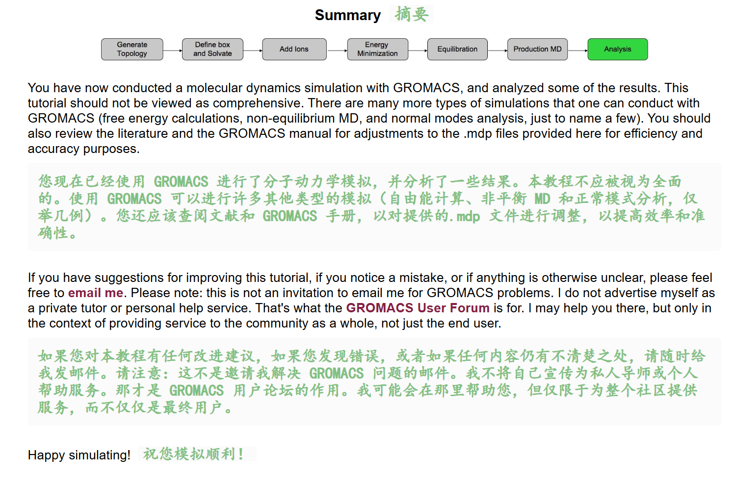
5,Energy Minimization 能量最小化
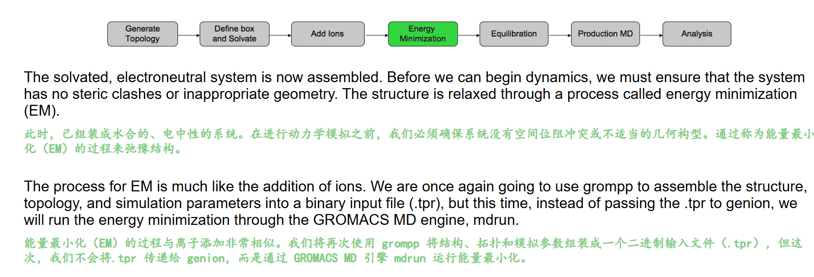
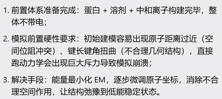
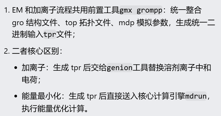
水合中性体系搭建好后不能直接动力学,原子空间挤压会报错,必须做能量最小化弛豫结构;该步骤前期打包文件的命令和加离子一致,只是后续调用程序不同,EM 直接用 mdrun 运算。
同样的,官方教程提供了1个能量最小化的md模拟参数文件
http://www.mdtutorials.com/gmx/lysozyme/Files/minim.mdp
粘贴如下
python
; minim.mdp - used as input into grompp to generate em.tpr
; Parameters describing what to do, when to stop and what to save
integrator  = steep         ; Algorithm (steep = steepest descent minimization)
emtol       = 1000.0        ; Stop minimization when the maximum force < 1000.0 kJ/mol/nm
emstep      = 0.01          ; Minimization step size
nsteps      = 50000         ; Maximum number of (minimization) steps to perform

; Parameters describing how to find the neighbors of each atom and how to calculate the interactions
nstlist         = 1         ; Frequency to update the neighbor list and long range forces
cutoff-scheme   = Verlet    ; Buffered neighbor searching
ns_type         = grid      ; Method to determine neighbor list (simple, grid)
coulombtype     = PME       ; Treatment of long range electrostatic interactions
rcoulomb        = 1.0       ; Short-range electrostatic cut-off
rvdw            = 1.0       ; Short-range Van der Waals cut-off
pbc             = xyz       ; Periodic Boundary Conditions in all 3 dimensions
同样注释如下
python
; minim.mdp - used as input into grompp to generate em.tpr
; 注释:能量最小化参数文件,给grompp生成能量最小化二进制文件em.tpr

; ========== 1. 能量最小化核心控制参数 ==========
integrator  = steep         ; 积分器算法:steep = 最陡下降法(EM专用)
emtol       = 1000.0        ; 收敛判据,单位 kJ/mol/nm
                            ; 当体系**最大原子受力** < 1000 时,自动停止最小化
emstep      = 0.01          ; 最小化初始步长,单位 nm;每次原子移动最大距离0.01nm
nsteps      = 50000         ; 最大迭代步数上限,最多跑5万步;提前满足emtol会自动终止

; ========== 2. 近邻列表 & 相互作用计算参数 ==========
nstlist         = 1         ; 每1步更新一次近邻原子列表(EM阶段原子位置变化大,频繁更新)
cutoff-scheme   = Verlet    ; Verlet缓冲近邻列表方案,现代GROMACS标准,速度更快、稳定
ns_type         = grid      ; 网格法查找近邻原子,大体系效率高
coulombtype     = PME       ; 长程静电作用用PME粒子网格埃瓦尔德,生物体系标准算法
rcoulomb        = 1.0       ; 短程静电截断半径1.0 nm,超过1nm用PME计算长程静电
rvdw            = 1.0       ; 范德华力截断半径1.0 nm,超过1nm不再直接计算
pbc             = xyz       ; x/y/z三维全部开启周期性边界条件,模拟无限水溶液盒子
整个命令如下
python
gmx grompp -f minim.mdp -c 1AKI_solv_ions.gro -p topol.top -o em.tpr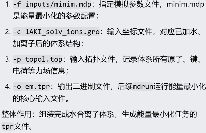
输出日志如下
python
Executable:   /home/csn/program/miniconda3/envs/tf-dna-md/bin.AVX2_256/gmx
Data prefix:  /home/csn/program/miniconda3/envs/tf-dna-md
Working dir:  /mnt/sdb/zht/project/tf-dna-md/files/structure
Command line:
  gmx grompp -f minim.mdp -c 1AKI_solv_ions.gro -p topol.top -o em.tpr

Ignoring obsolete mdp entry 'ns_type'

# mdp 写了 nstlist = 1,每一步更新近邻表
# GROMACS 提示:Verlet 方案下最优是 10 步以上更新,GPU 推荐 20;
# 关键:不影响计算精度,只会轻微降低计算速度
NOTE 1 [file minim.mdp]:
  With Verlet lists the optimal nstlist is >= 10, with GPUs >= 20. Note
  that with the Verlet scheme, nstlist has no effect on the accuracy of
  your simulation.

# ⚠️ 拓扑与力场参数加载
# 随机种子初始化完成
Setting the LD random seed to -336727121

# 非键相互作用、1-4 二面角作用参数全部成功匹配力场,无缺失参数报错;
Generated 169542 of the 169653 non-bonded parameter combinations
# fudge=1 是蛋白体系标准 1-4 缩放系数,正常
Generating 1-4 interactions: fudge = 1

Generated 118878 of the 169653 1-4 parameter combinations

# 分子内近邻排除设置
# 自动对蛋白、水、氯离子排除成键相邻原子的非键作用,力场规则匹配正确,无拓扑错误
Excluding 3 bonded neighbours molecule type 'Protein_chain_A'

Excluding 2 bonded neighbours molecule type 'SOL'

Excluding 3 bonded neighbours molecule type 'CL'

# 体系组分统计
Analysing residue names:
# 体系组成:129 个氨基酸蛋白 + 12589 个水分子 + 8 个氯离子,结构 / 拓扑匹配无误
There are:   129    Protein residues
There are: 12589      Water residues
There are:     8        Ion residues # 离子数量 = 8,对应上前面添加的8个氯离子
Analysing Protein...

# 控温、体系自由度相关
# 自由度正常计算
Number of degrees of freedom in T-Coupling group rest is 81435.00
# 提示无体系温度:因为当前是能量最小化(integrator=steep),最小化本身不需要温度,属于正常提示,不用处理
The integrator does not provide a ensemble temperature, there is no system ensemble temperature

# 原子排斥距离检查
# 排除原子最小间距 0.443 nm,没有出现原子极度重叠(<0.1 nm)的高危冲突,体系初始结构没有严重炸结构风险
The largest distance between excluded atoms is 0.443 nm between atom 1156 and 1405

# # PME 长程静电网格计算参数
Calculating fourier grid dimensions for X Y Z
# PME 傅里叶网格 64×64×64,网格间距 0.116 nm,精度满足生物模拟要求
Using a fourier grid of 64x64x64, spacing 0.116 0.116 0.116

# PME 计算负载仅占 25%,算力压力小,运行速度快
Estimate for the relative computational load of the PME mesh part: 0.25

# 最小化产生的日志、能量文件总大小约 3MB,体积很小
This run will generate roughly 3 Mb of data

There was 1 NOTE

GROMACS reminds you: "Sometimes Life is Obscene" (Black Crowes)
同样的,我们输入有mdp文件,
输出除了tpr文件之外,还有一个mdp文件
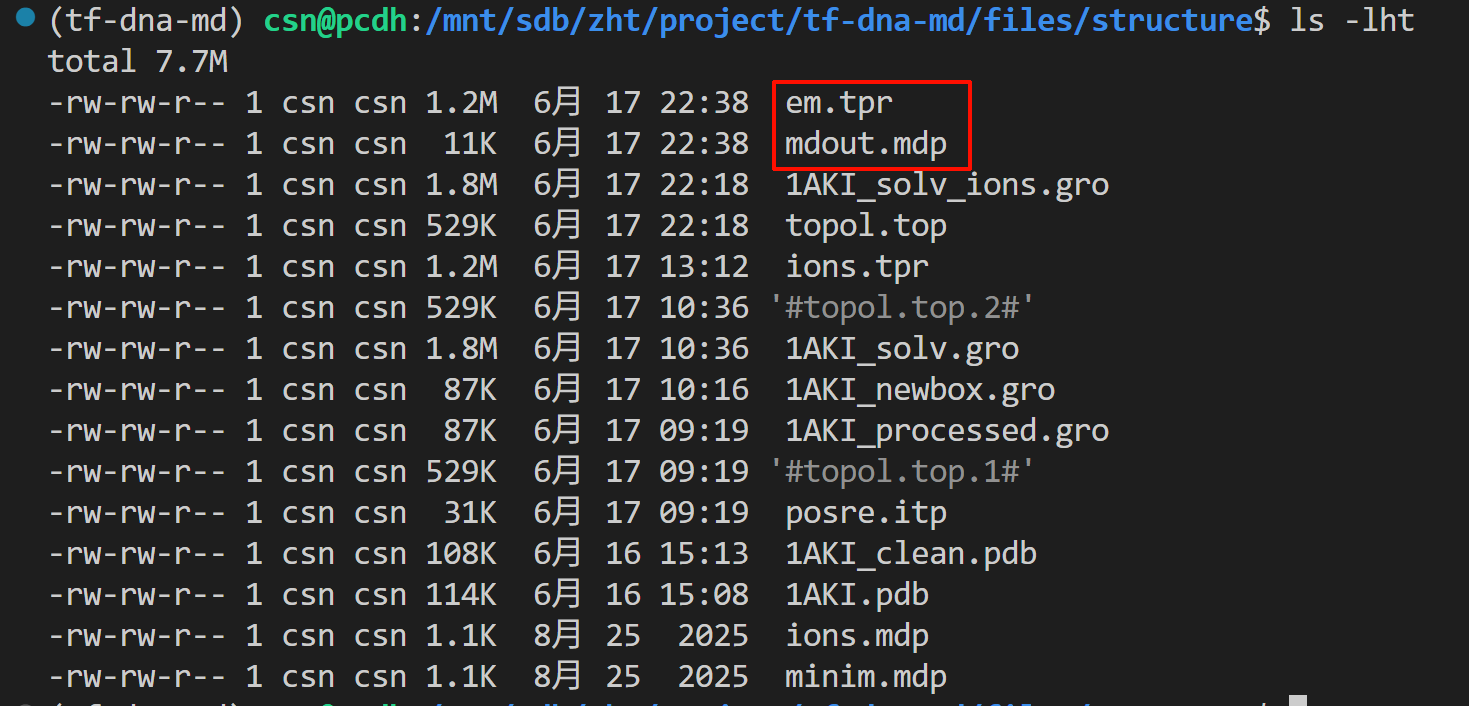
这里重申一下,mdout.mdp是gmx grompp运行成功后自动导出的完整标准版参数文件,和本次生成的tpr文件严格一一对应,记录了本次模拟所有实际生效的参数
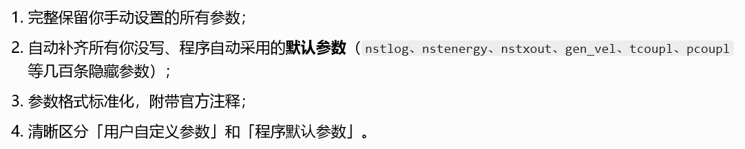
可以保证日后模拟可完全复现

⚠️ 因为后续还要跑NVT/NPT、生产MD,多阶段模拟的话每一次grompp都会覆盖mdout.mdp文件,所以建议是生成之后立刻重命名

接下来执行能量最小化,需要用到mdrun命令,
同样的,我们来查看一下这个命令
python
gmx mdrun
gmx help mdrun
python
Executable:   /home/csn/program/miniconda3/envs/tf-dna-md/bin.AVX2_256/gmx
Data prefix:  /home/csn/program/miniconda3/envs/tf-dna-md
Working dir:  /mnt/sdb/zht/project/tf-dna-md/files/structure
Command line:
  gmx help mdrun

SYNOPSIS

gmx mdrun [-s [<.tpr>]] [-cpi [<.cpt>]] [-table [<.xvg>]] [-tablep [<.xvg>]]
          [-tableb [<.xvg> [...]]] [-rerun [<.xtc/.trr/...>]] [-ei [<.edi>]]
          [-multidir [<dir> [...]]] [-awh [<.xvg>]] [-plumed [<.dat>]]
          [-membed [<.dat>]] [-mp [<.top>]] [-mn [<.ndx>]]
          [-o [<.trr/.cpt/...>]] [-x [<.xtc/.tng>]] [-cpo [<.cpt>]]
          [-c [<.gro/.g96/...>]] [-e [<.edr>]] [-g [<.log>]] [-dhdl [<.xvg>]]
          [-field [<.xvg>]] [-tpi [<.xvg>]] [-tpid [<.xvg>]] [-eo [<.xvg>]]
          [-px [<.xvg>]] [-pf [<.xvg>]] [-ro [<.xvg>]] [-ra [<.log>]]
          [-rs [<.log>]] [-rt [<.log>]] [-mtx [<.mtx>]] [-if [<.xvg>]]
          [-swap [<.xvg>]] [-deffnm <string>] [-xvg <enum>] [-dd <vector>]
          [-ddorder <enum>] [-npme <int>] [-nt <int>] [-ntmpi <int>]
          [-ntomp <int>] [-ntomp_pme <int>] [-pin <enum>] [-pinoffset <int>]
          [-pinstride <int>] [-gpu_id <string>] [-gputasks <string>]
          [-[no]ddcheck] [-rdd <real>] [-rcon <real>] [-dlb <enum>]
          [-dds <real>] [-nb <enum>] [-nstlist <int>] [-[no]tunepme]
          [-pme <enum>] [-pmefft <enum>] [-bonded <enum>] [-update <enum>]
          [-[no]v] [-pforce <real>] [-[no]reprod] [-cpt <real>] [-[no]cpnum]
          [-[no]append] [-nsteps <int>] [-maxh <real>] [-replex <int>]
          [-nex <int>] [-reseed <int>]

DESCRIPTION

gmx mdrun is the main computational chemistry engine within GROMACS.
Obviously, it performs Molecular Dynamics simulations, but it can also perform
Stochastic Dynamics, Energy Minimization, test particle insertion or
(re)calculation of energies. Normal mode analysis is another option. In this
case mdrun builds a Hessian matrix from single conformation. For usual Normal
Modes-like calculations, make sure that the structure provided is properly
energy-minimized. The generated matrix can be diagonalized by gmx nmeig.

The mdrun program reads the run input file (-s) and distributes the topology
over ranks if needed. mdrun produces at least four output files. A single log
file (-g) is written. The trajectory file (-o), contains coordinates,
velocities and optionally forces. The structure file (-c) contains the
coordinates and velocities of the last step. The energy file (-e) contains
energies, the temperature, pressure, etc, a lot of these things are also
printed in the log file. Optionally coordinates can be written to a compressed
trajectory file (-x).

The option -dhdl is only used when free energy calculation is turned on.

Running mdrun efficiently in parallel is a complex topic, many aspects of
which are covered in the online User Guide. You should look there for
practical advice on using many of the options available in mdrun.

ED (essential dynamics) sampling and/or additional flooding potentials are
switched on by using the -ei flag followed by an .edi file. The .edi file can
be produced with the make_edi tool or by using options in the essdyn menu of
the WHAT IF program. mdrun produces a .xvg output file that contains
projections of positions, velocities and forces onto selected eigenvectors.

When user-defined potential functions have been selected in the .mdp file the
-table option is used to pass mdrun a formatted table with potential
functions. The file is read from either the current directory or from the
GMXLIB directory. A number of pre-formatted tables are presented in the GMXLIB
dir, for 6-8, 6-9, 6-10, 6-11, 6-12 Lennard-Jones potentials with normal
Coulomb. When pair interactions are present, a separate table for pair
interaction functions is read using the -tablep option.

When tabulated bonded functions are present in the topology, interaction
functions are read using the -tableb option. For each different tabulated
interaction type used, a table file name must be given. For the topology to
work, a file name given here must match a character sequence before the file
extension. That sequence is: an underscore, then a 'b' for bonds, an 'a' for
angles or a 'd' for dihedrals, and finally the matching table number index
used in the topology. Note that, these options are deprecated, and in future
will be available via grompp.

The options -px and -pf are used for writing pull COM coordinates and forces
when pulling is selected in the .mdp file.

The option -membed does what used to be g_membed, i.e. embed a protein into a
membrane. This module requires a number of settings that are provided in a
data file that is the argument of this option. For more details in membrane
embedding, see the documentation in the user guide. The options -mn and -mp
are used to provide the index and topology files used for the embedding.

The option -pforce is useful when you suspect a simulation crashes due to too
large forces. With this option coordinates and forces of atoms with a force
larger than a certain value will be printed to stderr. It will also terminate
the run when non-finite forces are present.

Checkpoints containing the complete state of the system are written at regular
intervals (option -cpt) to the file -cpo, unless option -cpt is set to -1. The
previous checkpoint is backed up to state_prev.cpt to make sure that a recent
state of the system is always available, even when the simulation is
terminated while writing a checkpoint. With -cpnum all checkpoint files are
kept and appended with the step number. A simulation can be continued by
reading the full state from file with option -cpi. This option is intelligent
in the way that if no checkpoint file is found, GROMACS just assumes a normal
run and starts from the first step of the .tpr file. By default the output
will be appending to the existing output files. The checkpoint file contains
checksums of all output files, such that you will never loose data when some
output files are modified, corrupt or removed. There are three scenarios with
-cpi:

* no files with matching names are present: new output files are written

* all files are present with names and checksums matching those stored in the
checkpoint file: files are appended

* otherwise no files are modified and a fatal error is generated

With -noappend new output files are opened and the simulation part number is
added to all output file names. Note that in all cases the checkpoint file
itself is not renamed and will be overwritten, unless its name does not match
the -cpo option.

With checkpointing the output is appended to previously written output files,
unless -noappend is used or none of the previous output files are present
(except for the checkpoint file). The integrity of the files to be appended is
verified using checksums which are stored in the checkpoint file. This ensures
that output can not be mixed up or corrupted due to file appending. When only
some of the previous output files are present, a fatal error is generated and
no old output files are modified and no new output files are opened. The
result with appending will be the same as from a single run. The contents will
be binary identical, unless you use a different number of ranks or dynamic
load balancing or the FFT library uses optimizations through timing.

With option -maxh a simulation is terminated and a checkpoint file is written
at the first neighbor search step where the run time exceeds -maxh*0.99 hours.
This option is particularly useful in combination with setting nsteps to -1
either in the mdp or using the similarly named command line option (although
the latter is deprecated). This results in an infinite run, terminated only
when the time limit set by -maxh is reached (if any) or upon receiving a
signal.

Interactive molecular dynamics (IMD) can be activated by using at least one of
the three IMD switches: The -imdterm switch allows one to terminate the
simulation from the molecular viewer (e.g. VMD). With -imdwait, mdrun pauses
whenever no IMD client is connected. Pulling from the IMD remote can be turned
on by -imdpull. The port mdrun listens to can be altered by -imdport.The file
pointed to by -if contains atom indices and forces if IMD pulling is used.

OPTIONS

Options to specify input files:

 -s      [<.tpr>]           (topol.tpr)
           Portable xdr run input file
 -cpi    [<.cpt>]           (state.cpt)      (Opt.)
           Checkpoint file
 -table  [<.xvg>]           (table.xvg)      (Opt.)
           xvgr/xmgr file
 -tablep [<.xvg>]           (tablep.xvg)     (Opt.)
           xvgr/xmgr file
 -tableb [<.xvg> [...]]     (table.xvg)      (Opt.)
           xvgr/xmgr file
 -rerun  [<.xtc/.trr/...>]  (rerun.xtc)      (Opt.)
           Trajectory: xtc trr cpt gro g96 pdb tng
 -ei     [<.edi>]           (sam.edi)        (Opt.)
           ED sampling input
 -multidir [<dir> [...]]    (rundir)         (Opt.)
           Run directory
 -awh    [<.xvg>]           (awhinit.xvg)    (Opt.)
           xvgr/xmgr file
 -plumed [<.dat>]           (plumed.dat)     (Opt.)
           Generic data file
 -membed [<.dat>]           (membed.dat)     (Opt.)
           Generic data file
 -mp     [<.top>]           (membed.top)     (Opt.)
           Topology file
 -mn     [<.ndx>]           (membed.ndx)     (Opt.)
           Index file

Options to specify output files:

 -o      [<.trr/.cpt/...>]  (traj.trr)
           Full precision trajectory: trr cpt tng
 -x      [<.xtc/.tng>]      (traj_comp.xtc)  (Opt.)
           Compressed trajectory (tng format or portable xdr format)
 -cpo    [<.cpt>]           (state.cpt)      (Opt.)
           Checkpoint file
 -c      [<.gro/.g96/...>]  (confout.gro)
           Structure file: gro g96 pdb brk ent esp
 -e      [<.edr>]           (ener.edr)
           Energy file
 -g      [<.log>]           (md.log)
           Log file
 -dhdl   [<.xvg>]           (dhdl.xvg)       (Opt.)
           xvgr/xmgr file
 -field  [<.xvg>]           (field.xvg)      (Opt.)
           xvgr/xmgr file
 -tpi    [<.xvg>]           (tpi.xvg)        (Opt.)
           xvgr/xmgr file
 -tpid   [<.xvg>]           (tpidist.xvg)    (Opt.)
           xvgr/xmgr file
 -eo     [<.xvg>]           (edsam.xvg)      (Opt.)
           xvgr/xmgr file
 -px     [<.xvg>]           (pullx.xvg)      (Opt.)
           xvgr/xmgr file
 -pf     [<.xvg>]           (pullf.xvg)      (Opt.)
           xvgr/xmgr file
 -ro     [<.xvg>]           (rotation.xvg)   (Opt.)
           xvgr/xmgr file
 -ra     [<.log>]           (rotangles.log)  (Opt.)
           Log file
 -rs     [<.log>]           (rotslabs.log)   (Opt.)
           Log file
 -rt     [<.log>]           (rottorque.log)  (Opt.)
           Log file
 -mtx    [<.mtx>]           (nm.mtx)         (Opt.)
           Hessian matrix
 -if     [<.xvg>]           (imdforces.xvg)  (Opt.)
           xvgr/xmgr file
 -swap   [<.xvg>]           (swapions.xvg)   (Opt.)
           xvgr/xmgr file

Other options:

 -deffnm <string>
           Set the default filename for all file options
 -xvg    <enum>             (xmgrace)
           xvg plot formatting: xmgrace, xmgr, none
 -dd     <vector>           (0 0 0)
           Domain decomposition grid, 0 is optimize
 -ddorder <enum>            (interleave)
           DD rank order: interleave, pp_pme, cartesian
 -npme   <int>              (-1)
           Number of separate ranks to be used for PME, -1 is guess
 -nt     <int>              (0)
           Total number of threads to start (0 is guess)
 -ntmpi  <int>              (0)
           Number of thread-MPI ranks to start (0 is guess)
 -ntomp  <int>              (0)
           Number of OpenMP threads per MPI rank to start (0 is guess)
 -ntomp_pme <int>           (0)
           Number of OpenMP threads per MPI rank to start (0 is -ntomp)
 -pin    <enum>             (auto)
           Whether mdrun should try to set thread affinities: auto, on, off
 -pinoffset <int>           (0)
           The lowest logical core number to which mdrun should pin the first
           thread
 -pinstride <int>           (0)
           Pinning distance in logical cores for threads, use 0 to minimize
           the number of threads per physical core
 -gpu_id <string>
           List of unique GPU device IDs available to use
 -gputasks <string>
           List of GPU device IDs, mapping each task on a node to a device.
           Tasks include PP and PME (if present).
 -[no]ddcheck               (yes)
           Check for all bonded interactions with DD
 -rdd    <real>             (0)
           The maximum distance for bonded interactions with DD (nm), 0 is
           determine from initial coordinates
 -rcon   <real>             (0)
           Maximum distance for P-LINCS (nm), 0 is estimate
 -dlb    <enum>             (auto)
           Dynamic load balancing (with DD): auto, no, yes
 -dds    <real>             (0.8)
           Fraction in (0,1) by whose reciprocal the initial DD cell size will
           be increased in order to provide a margin in which dynamic load
           balancing can act while preserving the minimum cell size.
 -nb     <enum>             (auto)
           Calculate non-bonded interactions on: auto, cpu, gpu
 -nstlist <int>             (0)
           Set nstlist when using a Verlet buffer tolerance (0 is guess)
 -[no]tunepme               (yes)
           Optimize PME load between PP/PME ranks or GPU/CPU
 -pme    <enum>             (auto)
           Perform PME calculations on: auto, cpu, gpu
 -pmefft <enum>             (auto)
           Perform PME FFT calculations on: auto, cpu, gpu
 -bonded <enum>             (auto)
           Perform bonded calculations on: auto, cpu, gpu
 -update <enum>             (auto)
           Perform update and constraints on: auto, cpu, gpu
 -[no]v                     (no)
           Be loud and noisy
 -pforce <real>             (-1)
           Print all forces larger than this (kJ/mol nm)
 -[no]reprod                (no)
           Avoid optimizations that affect binary reproducibility; this can
           significantly reduce performance
 -cpt    <real>             (15)
           Checkpoint interval (minutes)
 -[no]cpnum                 (no)
           Keep and number checkpoint files
 -[no]append                (yes)
           Append to previous output files when continuing from checkpoint
           instead of adding the simulation part number to all file names
 -nsteps <int>              (-2)
           Run this number of steps (-1 means infinite, -2 means use mdp
           option, smaller is invalid)
 -maxh   <real>             (-1)
           Terminate after 0.99 times this time (hours)
 -replex <int>              (0)
           Attempt replica exchange periodically with this period (steps)
 -nex    <int>              (0)
           Number of random exchanges to carry out each exchange interval (N^3
           is one suggestion).  -nex zero or not specified gives neighbor
           replica exchange.
 -reseed <int>              (-1)
           Seed for replica exchange, -1 is generate a seed

GROMACS reminds you: "Always code as if the person who ends up maintaining your code is a violent psychopath who knows where you live." (Martin Golding)
mdrun是核心的一个子命令,
一、程序整体定位
gmx mdrun 是 GROMACS唯一核心计算引擎,所有分子模拟计算均由它执行:
- 常规模拟:NVT/NPT/NVE分子动力学、能量最小化EM、随机动力学SD
- 进阶计算:自由能、副本交换REMD、PLUMED增强采样、轨迹重计算、简正模式NMA、拉伸模拟、蛋白膜嵌入
- 输入前提:必须先用
gmx grompp编译生成.tpr文件(包含拓扑、模拟参数、初坐标/速度),无tpr无法运行。
二、输入文件参数(高频)
必选输入
-s [topol.tpr]
全局唯一必填参数,二进制运行文件,存储整套体系与mdp模拟设置。
续跑核心输入(超算最常用)
-cpi [state.cpt]
读取检查点完整系统状态(坐标、速度、温压耦合、随机种子)实现断点续跑;无cpt文件则从头启动模拟。
进阶输入
-plumed plumed.dat:耦合PLUMED,元动力学/伞形采样等自由能增强采样标配-rerun traj.xtc:轨迹重算,不积分运动方程,仅基于已有轨迹重新计算能量、受力-multidir dir1 dir2:一次性运行多副本,副本交换专用-ei sam.edi:主成分(ED)采样,用于构象空间约束采样
专用输入
-table/tablep/tableb:自定义LJ/键合查表势,自研力场才会用到-membed / -mp / -mn:自动将蛋白嵌入磷脂膜,膜模拟专用
三、输出文件参数(日常模拟)
基础默认输出(每次模拟都会生成)
-o traj.trr:高精度完整轨迹(坐标+速度+受力,体积大)-x traj_comp.xtc:压缩坐标轨迹,可视化、后处理首选,占用空间小-c confout.gro:模拟最后一帧结构,用于提取终态构象-e ener.edr:能量文件,存储温度、压强、势能、盒尺寸等,用gmx energy分析-g md.log:日志文件,报错、性能、每步能量全部记录,排错第一文件
续跑关键输出
-cpo state.cpt
定时写入完整检查点,断电/队列超时后依靠 -cpi 续跑。
专项输出
-dhdl dhdl.xvg:自由能模拟专属,记录λ相关能量差-px / -pf pullx.xvg pullf.xvg:拉伸模拟,输出质心距离、拉力曲线-pforce X:崩溃排查工具,打印所有受力>X kJ/(mol·nm) 的原子,快速定位爆炸位点-mtx nm.mtx:简正模式NMA输出海森矩阵,需搭配gmx nmeig对角化
极简统一文件名(高频实用参数)
-deffnm md
一键统一所有输入输出前缀:md.tpr、md.xtc、md.log、md.cpt,无需逐个指定-o/-x/-g,日常模拟必用。
四、并行 & GPU 性能调参(集群/显卡模拟核心)
1. CPU线程/MPI分配
-ntmpi N:MPI进程数,负责域分解PP、PME任务拆分-ntomp M:单个MPI进程内OpenMP线程数;总CPU核数 = ntmpi × ntomp-nt:总线程自动拆分,不推荐手动设置,集群建议精确控制ntmpi/ntomp-ntomp_pme:PME长程静电单独分配线程,默认同ntomp
2. GPU调度(带显卡服务器刚需)
-gpu_id 0,1:指定使用的显卡编号,多卡模拟分配设备-nb auto/cpu/gpu:非键相互作用计算设备,auto自动跑GPU-pme / -bonded / -update:长程静电、键合作用、运动积分设备,auto优先GPU加速-gputasks:精细绑定MPI任务与显卡,多复本均衡负载
3. 域分解DD(大体系并行加速)
-dd X Y Z:手动设置三维分解网格,0 0 0程序自动优化(默认)-dlb auto/yes/no:动态负载均衡,大分子/不均一体系建议开启,平衡各硬件计算量-npme N:单独分出N个MPI进程专门计算PME,超大体系显著提速-ddcheck:校验跨域成键完整性,默认开启
五、模拟时长 & 检查点 & 续跑控制(超算队列必备)
1. 总步数控制
-nsteps N
-2(默认):读取mdp文件内设置的总步数-1:无限循环运行,配合-maxh实现限时模拟
2. 限时自动安全退出(队列神器)
-maxh 23.5
运行时长达到设定值99%时,自动写入检查点并终止,适配24h队列时限,避免数据丢失。
3. 检查点配置
-cpt 15:默认每15分钟写入一次cpt(单位:分钟),可缩短至5/10分钟防断电-cpnum:保存全部历史检查点(state_0.cpt、state_1.cpt),不覆盖,可回溯任意中间帧-noappend:续跑不追加旧轨迹,生成带编号新文件(md_part0002.xtc);默认-append直接追加到原有轨迹
4. -cpi 续跑内置校验逻辑(防数据错乱)
- 无旧输出文件:全新模拟,生成全套新文件
- 旧文件齐全且校验和匹配:直接追加续写
- 文件缺失/损坏:直接报错终止,禁止混合新旧数据
六、高级特色功能参数
- 副本交换REMD
-replex N:每N步尝试一次复本交换;-nex控制单次交换尝试数量 - PLUMED增强采样
-plumed dat,自由能、约束、元动力学模拟标配 - 简正模式NMA
搭配-mtx输出海森矩阵,要求体系提前能量极小化 - IMD实时交互(VMD联动)
-imdwait/-imdterm/-imdpull,可视化实时观测正在运行的模拟、实时施加外力 - 轨迹重计算 rerun
-rerun 轨迹文件,修改力场/温度后批量重新计算能量,不消耗动力学积分算力
七、高频实操最简命令示例
- 常规单卡MD(推荐写法)
bash
gmx mdrun -deffnm md -s md.tpr -gpu_id 0 -ntmpi 4 -ntomp 6- 队列超时断点续跑
bash
gmx mdrun -deffnm md -s md.tpr -cpi md.cpt -gpu_id 0- 24h限时无限长模拟
bash
gmx mdrun -deffnm md -s md.tpr -nsteps -1 -maxh 23.8 -cpt 10- 轨迹重算能量
bash
gmx mdrun -s md.tpr -rerun traj.xtc -deffnm rerun- 排查模拟崩溃(打印受力爆炸原子)
bash
gmx mdrun -deffnm md -s md.tpr -pforce 1000- 耦合PLUMED元动力学
bash
gmx mdrun -deffnm meta -s meta.tpr -plumed plumed.dat -gpu_id 0核心重点
- -deffnm 是最实用参数,统一全部文件前缀,简化命令;
.tpr是模拟基准,修改mdp/拓扑后必须重新grompp,续跑不会读取新参数;-cpt + -cpi + -maxh三组合是超算长时模拟续命核心,防止队列截断丢数据;- GPU模拟无需复杂设置,仅
-gpu_id指定卡号,其余计算设备默认auto自动加速; - 并行分配规则:
ntmpi控制域分解进程,ntomp单进程线程,总核数=两者乘积;大体系加-npme加速PME; - 模拟崩溃排查顺序:先看
md.log日志,其次加-pforce定位受力异常原子; - 默认开启
-append续跑追加轨迹,内置文件校验和,旧轨迹损坏会直接报错,不会污染数据; -nsteps -1搭配-maxh是无限时长模拟标准方案,适配超算队列时间限制;-rerun仅重算能量,不跑动力学,算力消耗极低,适合批量后处理。
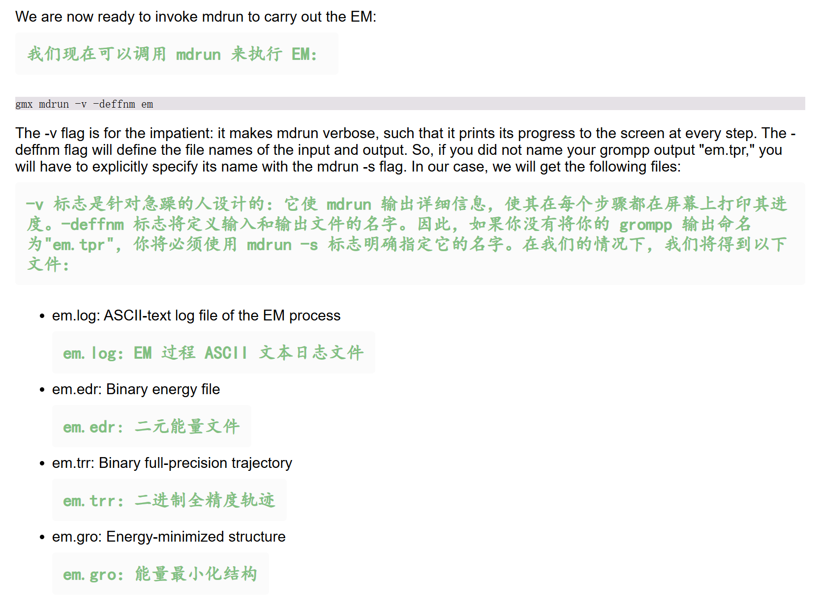
然后我们现在运行的程序如下:
python
gmx mdrun -v -deffnm em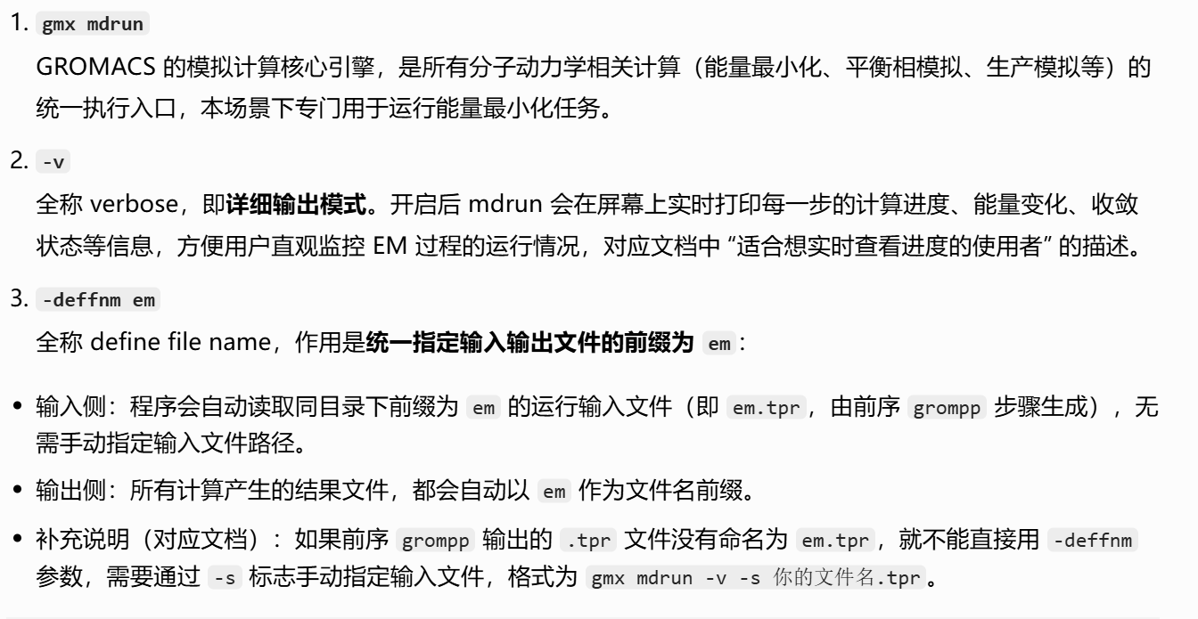
这一步,就是基于前置步骤 grompp 生成的拓扑输入文件,通过算法迭代降低体系势能、消除不合理的原子接触,最终输出能量稳定的优化后分子结构
输出日志粘贴如下,一并中文注释
python
# ⚠️ 最陡下降法能量最小化(EM)的完整运行过程
Executable: /home/csn/program/miniconda3/envs/tf-dna-md/bin.AVX2_256/gmx
Data prefix: /home/csn/program/miniconda3/envs/tf-dna-md
Working dir: /mnt/sdb/zht/project/tf-dna-md/files/structure
Command line:
gmx mdrun -v -deffnm em
# 硬件优化提示
# ⚠️ 当前编译使用 AVX2_256 指令集,但我们的 CPU 支持 AVX_512 指令集,重新编译并启用 AVX512 可进一步提升计算速度
Compiled SIMD is AVX2_256, but AVX_512 might be faster (see log).
# CPU 计时精度高于程序编译默认配置,建议开启 GMX_USE_RDTSCP 编译选项优化负载均衡
The current CPU can measure timings more accurately than the code in
gmx mdrun was configured to use. This might affect your simulation
speed as accurate timings are needed for load-balancing.
Please consider rebuilding gmx mdrun with the GMX_USE_RDTSCP=ON CMake option.
Reading file em.tpr, VERSION 2025.4-conda_forge (single precision)
# 并行设置:启用 32 个 MPI 线程,每个 MPI 线程绑定 1 个 OpenMP 线程
Using 32 MPI threads
Using 1 OpenMP thread per tMPI thread
# ⚠️ 能量最小化核心参数
# 算法:最陡下降法(Steepest Descents),适合初步快速消除体系不合理接触、大幅降低势能
Steepest Descents:
# 收敛判据:单个原子的最大受力 Fmax < 1000 kJ/(mol·nm)
Tolerance (Fmax) = 1.00000e+03
# 迭代步数上限:50000 步
Number of steps = 50000
# 迭代过程与趋势
# 初始状态(第 0 步)
# 体系势能为 -4.56762×10⁵ kJ/mol,最大受力高达 1.81×10⁵ kJ/(mol·nm),受力集中在 1891 号原子,说明初始结构存在明显的不合理原子重叠 / 接触。
# 优化趋势
# 迭代过程中势能持续单调下降,最大受力整体逐步降低;算法会自动调整单步最大位移(Dmax),前期步长较大以快速降低势能,后期步长收窄以精细优化结构。
# 最大受力对应的原子从 1891 号依次转移到 934 号、567 号,反映体系不同区域的不合理接触被依次消除。
Step= 0, Dmax= 1.0e-02 nm, Epot= -4.56762e+05 Fmax= 1.81019e+05, atom= 1891
Step= 1, Dmax= 1.0e-02 nm, Epot= -4.68770e+05 Fmax= 6.69897e+04, atom= 936
Step= 2, Dmax= 1.2e-02 nm, Epot= -4.82035e+05 Fmax= 2.92863e+04, atom= 19484
Step= 3, Dmax= 1.4e-02 nm, Epot= -4.94717e+05 Fmax= 1.37512e+04, atom= 19484
Step= 4, Dmax= 1.7e-02 nm, Epot= -5.07843e+05 Fmax= 6.31431e+03, atom= 19484
Step= 5, Dmax= 2.1e-02 nm, Epot= -5.22318e+05 Fmax= 5.89126e+03, atom= 934
Step= 6, Dmax= 2.5e-02 nm, Epot= -5.28868e+05 Fmax= 2.44084e+04, atom= 934
Step= 7, Dmax= 3.0e-02 nm, Epot= -5.34062e+05 Fmax= 1.51313e+04, atom= 934
Step= 9, Dmax= 1.8e-02 nm, Epot= -5.36844e+05 Fmax= 8.52869e+03, atom= 934
Step= 10, Dmax= 2.1e-02 nm, Epot= -5.39044e+05 Fmax= 2.10623e+04, atom= 934
Step= 11, Dmax= 2.6e-02 nm, Epot= -5.41936e+05 Fmax= 1.35461e+04, atom= 934
Step= 12, Dmax= 3.1e-02 nm, Epot= -5.42092e+05 Fmax= 2.89545e+04, atom= 934
Step= 13, Dmax= 3.7e-02 nm, Epot= -5.45300e+05 Fmax= 2.12184e+04, atom= 934
Step= 15, Dmax= 2.2e-02 nm, Epot= -5.48040e+05 Fmax= 8.96469e+03, atom= 934
Step= 16, Dmax= 2.7e-02 nm, Epot= -5.48530e+05 Fmax= 2.66611e+04, atom= 934
Step= 17, Dmax= 3.2e-02 nm, Epot= -5.51472e+05 Fmax= 1.68183e+04, atom= 934
Step= 19, Dmax= 1.9e-02 nm, Epot= -5.53318e+05 Fmax= 9.11460e+03, atom= 934
Step= 20, Dmax= 2.3e-02 nm, Epot= -5.53866e+05 Fmax= 2.25026e+04, atom= 934
Step= 21, Dmax= 2.8e-02 nm, Epot= -5.55970e+05 Fmax= 1.49228e+04, atom= 934
Step= 23, Dmax= 1.7e-02 nm, Epot= -5.57485e+05 Fmax= 7.60326e+03, atom= 934
Step= 24, Dmax= 2.0e-02 nm, Epot= -5.58210e+05 Fmax= 1.90640e+04, atom= 934
Step= 25, Dmax= 2.4e-02 nm, Epot= -5.59827e+05 Fmax= 1.33437e+04, atom= 934
Step= 27, Dmax= 1.4e-02 nm, Epot= -5.61117e+05 Fmax= 6.00747e+03, atom= 934
Step= 28, Dmax= 1.7e-02 nm, Epot= -5.61901e+05 Fmax= 1.75160e+04, atom= 934
Step= 29, Dmax= 2.1e-02 nm, Epot= -5.63411e+05 Fmax= 1.03830e+04, atom= 934
Step= 31, Dmax= 1.2e-02 nm, Epot= -5.64390e+05 Fmax= 6.42087e+03, atom= 934
Step= 32, Dmax= 1.5e-02 nm, Epot= -5.65116e+05 Fmax= 1.35153e+04, atom= 934
Step= 33, Dmax= 1.8e-02 nm, Epot= -5.66125e+05 Fmax= 1.06540e+04, atom= 934
Step= 34, Dmax= 2.1e-02 nm, Epot= -5.66228e+05 Fmax= 1.81875e+04, atom= 1171
Step= 35, Dmax= 2.6e-02 nm, Epot= -5.67168e+05 Fmax= 1.65981e+04, atom= 1171
Step= 37, Dmax= 1.5e-02 nm, Epot= -5.68775e+05 Fmax= 4.44978e+03, atom= 1694
Step= 38, Dmax= 1.9e-02 nm, Epot= -5.69068e+05 Fmax= 2.05716e+04, atom= 1694
Step= 39, Dmax= 2.2e-02 nm, Epot= -5.70949e+05 Fmax= 9.88074e+03, atom= 1694
Step= 41, Dmax= 1.3e-02 nm, Epot= -5.71657e+05 Fmax= 8.31493e+03, atom= 1694
Step= 42, Dmax= 1.6e-02 nm, Epot= -5.72051e+05 Fmax= 1.37515e+04, atom= 1694
Step= 43, Dmax= 1.9e-02 nm, Epot= -5.72760e+05 Fmax= 1.24526e+04, atom= 1694
Step= 44, Dmax= 2.3e-02 nm, Epot= -5.72786e+05 Fmax= 1.93468e+04, atom= 1694
Step= 45, Dmax= 2.8e-02 nm, Epot= -5.73477e+05 Fmax= 1.83709e+04, atom= 1694
Step= 47, Dmax= 1.7e-02 nm, Epot= -5.74905e+05 Fmax= 4.23850e+03, atom= 1694
Step= 48, Dmax= 2.0e-02 nm, Epot= -5.75038e+05 Fmax= 2.27359e+04, atom= 1694
Step= 49, Dmax= 2.4e-02 nm, Epot= -5.76763e+05 Fmax= 9.89265e+03, atom= 1694
Step= 51, Dmax= 1.4e-02 nm, Epot= -5.77274e+05 Fmax= 9.65416e+03, atom= 1694
Step= 52, Dmax= 1.7e-02 nm, Epot= -5.77578e+05 Fmax= 1.39882e+04, atom= 1694
Step= 53, Dmax= 2.1e-02 nm, Epot= -5.78045e+05 Fmax= 1.41553e+04, atom= 1694
Step= 54, Dmax= 2.5e-02 nm, Epot= -5.78072e+05 Fmax= 1.99350e+04, atom= 1694
Step= 55, Dmax= 3.0e-02 nm, Epot= -5.78458e+05 Fmax= 2.05613e+04, atom= 1694
Step= 57, Dmax= 1.8e-02 nm, Epot= -5.79875e+05 Fmax= 3.66749e+03, atom= 1694
Step= 59, Dmax= 1.1e-02 nm, Epot= -5.80452e+05 Fmax= 1.09586e+04, atom= 1694
Step= 60, Dmax= 1.3e-02 nm, Epot= -5.81003e+05 Fmax= 6.57583e+03, atom= 1694
Step= 61, Dmax= 1.5e-02 nm, Epot= -5.81219e+05 Fmax= 1.43604e+04, atom= 1694
Step= 62, Dmax= 1.9e-02 nm, Epot= -5.81816e+05 Fmax= 1.09413e+04, atom= 1694
Step= 64, Dmax= 1.1e-02 nm, Epot= -5.82361e+05 Fmax= 4.25790e+03, atom= 1694
Step= 65, Dmax= 1.3e-02 nm, Epot= -5.82735e+05 Fmax= 1.40571e+04, atom= 1694
Step= 66, Dmax= 1.6e-02 nm, Epot= -5.83374e+05 Fmax= 7.82219e+03, atom= 1694
Step= 68, Dmax= 9.6e-03 nm, Epot= -5.83767e+05 Fmax= 5.29561e+03, atom= 1694
Step= 69, Dmax= 1.2e-02 nm, Epot= -5.84108e+05 Fmax= 1.03756e+04, atom= 1694
Step= 70, Dmax= 1.4e-02 nm, Epot= -5.84520e+05 Fmax= 8.52991e+03, atom= 1694
Step= 71, Dmax= 1.7e-02 nm, Epot= -5.84677e+05 Fmax= 1.40118e+04, atom= 1694
Step= 72, Dmax= 2.0e-02 nm, Epot= -5.85068e+05 Fmax= 1.32274e+04, atom= 1694
Step= 74, Dmax= 1.2e-02 nm, Epot= -5.85670e+05 Fmax= 3.14998e+03, atom= 1694
Step= 75, Dmax= 1.4e-02 nm, Epot= -5.86094e+05 Fmax= 1.65425e+04, atom= 1694
Step= 76, Dmax= 1.7e-02 nm, Epot= -5.86825e+05 Fmax= 7.02862e+03, atom= 1694
Step= 78, Dmax= 1.0e-02 nm, Epot= -5.87136e+05 Fmax= 7.09256e+03, atom= 1694
Step= 79, Dmax= 1.2e-02 nm, Epot= -5.87399e+05 Fmax= 9.78092e+03, atom= 1694
Step= 80, Dmax= 1.5e-02 nm, Epot= -5.87679e+05 Fmax= 1.05639e+04, atom= 1694
Step= 81, Dmax= 1.8e-02 nm, Epot= -5.87848e+05 Fmax= 1.37045e+04, atom= 1694
Step= 82, Dmax= 2.1e-02 nm, Epot= -5.88043e+05 Fmax= 1.56069e+04, atom= 1694
Step= 83, Dmax= 2.6e-02 nm, Epot= -5.88068e+05 Fmax= 1.92981e+04, atom= 1694
Step= 85, Dmax= 1.5e-02 nm, Epot= -5.89038e+05 Fmax= 1.61936e+03, atom= 5674
Step= 86, Dmax= 1.8e-02 nm, Epot= -5.89805e+05 Fmax= 2.36244e+04, atom= 567
Step= 87, Dmax= 2.2e-02 nm, Epot= -5.91209e+05 Fmax= 7.06036e+03, atom= 567
Step= 89, Dmax= 1.3e-02 nm, Epot= -5.91362e+05 Fmax= 1.14370e+04, atom= 567
Step= 90, Dmax= 1.6e-02 nm, Epot= -5.91639e+05 Fmax= 1.05297e+04, atom= 567
Step= 91, Dmax= 1.9e-02 nm, Epot= -5.91659e+05 Fmax= 1.60321e+04, atom= 567
Step= 92, Dmax= 2.3e-02 nm, Epot= -5.91925e+05 Fmax= 1.55443e+04, atom= 567
Step= 94, Dmax= 1.4e-02 nm, Epot= -5.92512e+05 Fmax= 3.37904e+03, atom= 567
Step= 95, Dmax= 1.7e-02 nm, Epot= -5.92596e+05 Fmax= 1.94493e+04, atom= 567
Step= 96, Dmax= 2.0e-02 nm, Epot= -5.93341e+05 Fmax= 7.90612e+03, atom= 567
Step= 98, Dmax= 1.2e-02 nm, Epot= -5.93551e+05 Fmax= 8.48987e+03, atom= 567
Step= 99, Dmax= 1.4e-02 nm, Epot= -5.93710e+05 Fmax= 1.12018e+04, atom= 567
Step= 100, Dmax= 1.7e-02 nm, Epot= -5.93888e+05 Fmax= 1.23565e+04, atom= 567
Step= 101, Dmax= 2.1e-02 nm, Epot= -5.93959e+05 Fmax= 1.60858e+04, atom= 567
Step= 102, Dmax= 2.5e-02 nm, Epot= -5.94082e+05 Fmax= 1.77787e+04, atom= 567
Step= 104, Dmax= 1.5e-02 nm, Epot= -5.94715e+05 Fmax= 2.51174e+03, atom= 567
Step= 105, Dmax= 1.8e-02 nm, Epot= -5.94895e+05 Fmax= 2.21926e+04, atom= 567
Step= 106, Dmax= 2.1e-02 nm, Epot= -5.95746e+05 Fmax= 7.22105e+03, atom= 567
Step= 108, Dmax= 1.3e-02 nm, Epot= -5.95892e+05 Fmax= 1.03460e+04, atom= 567
Step= 109, Dmax= 1.5e-02 nm, Epot= -5.96071e+05 Fmax= 1.08216e+04, atom= 567
Step= 110, Dmax= 1.8e-02 nm, Epot= -5.96147e+05 Fmax= 1.44489e+04, atom= 567
Step= 111, Dmax= 2.2e-02 nm, Epot= -5.96273e+05 Fmax= 1.61000e+04, atom= 567
Step= 113, Dmax= 1.3e-02 nm, Epot= -5.96760e+05 Fmax= 2.25621e+03, atom= 567
Step= 114, Dmax= 1.6e-02 nm, Epot= -5.97125e+05 Fmax= 1.94982e+04, atom= 567
Step= 115, Dmax= 1.9e-02 nm, Epot= -5.97689e+05 Fmax= 6.89937e+03, atom= 567
Step= 117, Dmax= 1.1e-02 nm, Epot= -5.97844e+05 Fmax= 8.95981e+03, atom= 567
Step= 118, Dmax= 1.4e-02 nm, Epot= -5.97998e+05 Fmax= 9.96080e+03, atom= 567
Step= 119, Dmax= 1.7e-02 nm, Epot= -5.98111e+05 Fmax= 1.28670e+04, atom= 567
Step= 120, Dmax= 2.0e-02 nm, Epot= -5.98236e+05 Fmax= 1.43290e+04, atom= 567
Step= 121, Dmax= 2.4e-02 nm, Epot= -5.98264e+05 Fmax= 1.85757e+04, atom= 567
Step= 122, Dmax= 2.9e-02 nm, Epot= -5.98338e+05 Fmax= 2.05046e+04, atom= 567
Step= 124, Dmax= 1.7e-02 nm, Epot= -5.98926e+05 Fmax= 2.90986e+03, atom= 567
Step= 126, Dmax= 1.0e-02 nm, Epot= -5.99168e+05 Fmax= 1.14232e+04, atom= 567
Step= 127, Dmax= 1.2e-02 nm, Epot= -5.99402e+05 Fmax= 5.48975e+03, atom= 567
Step= 128, Dmax= 1.5e-02 nm, Epot= -5.99465e+05 Fmax= 1.47711e+04, atom= 567
Step= 129, Dmax= 1.8e-02 nm, Epot= -5.99740e+05 Fmax= 9.64621e+03, atom= 567
Step= 131, Dmax= 1.1e-02 nm, Epot= -5.99934e+05 Fmax= 5.02501e+03, atom= 567
Step= 132, Dmax= 1.3e-02 nm, Epot= -6.00045e+05 Fmax= 1.25462e+04, atom= 567
Step= 133, Dmax= 1.5e-02 nm, Epot= -6.00265e+05 Fmax= 8.54112e+03, atom= 567
Step= 135, Dmax= 9.2e-03 nm, Epot= -6.00437e+05 Fmax= 4.08106e+03, atom= 567
Step= 136, Dmax= 1.1e-02 nm, Epot= -6.00587e+05 Fmax= 1.11087e+04, atom= 567
Step= 137, Dmax= 1.3e-02 nm, Epot= -6.00786e+05 Fmax= 7.11694e+03, atom= 567
Step= 138, Dmax= 1.6e-02 nm, Epot= -6.00820e+05 Fmax= 1.46589e+04, atom= 567
Step= 139, Dmax= 1.9e-02 nm, Epot= -6.01038e+05 Fmax= 1.16270e+04, atom= 567
Step= 141, Dmax= 1.1e-02 nm, Epot= -6.01261e+05 Fmax= 4.15731e+03, atom= 567
Step= 142, Dmax= 1.4e-02 nm, Epot= -6.01362e+05 Fmax= 1.47328e+04, atom= 567
Step= 143, Dmax= 1.7e-02 nm, Epot= -6.01629e+05 Fmax= 7.95308e+03, atom= 567
Step= 145, Dmax= 9.9e-03 nm, Epot= -6.01778e+05 Fmax= 5.63057e+03, atom= 567
Step= 146, Dmax= 1.2e-02 nm, Epot= -6.01885e+05 Fmax= 1.06772e+04, atom= 567
Step= 147, Dmax= 1.4e-02 nm, Epot= -6.02043e+05 Fmax= 8.92857e+03, atom= 567
Step= 148, Dmax= 1.7e-02 nm, Epot= -6.02079e+05 Fmax= 1.44821e+04, atom= 567
Step= 149, Dmax= 2.1e-02 nm, Epot= -6.02230e+05 Fmax= 1.37951e+04, atom= 567
Step= 151, Dmax= 1.2e-02 nm, Epot= -6.02492e+05 Fmax= 3.18782e+03, atom= 567
Step= 152, Dmax= 1.5e-02 nm, Epot= -6.02620e+05 Fmax= 1.70802e+04, atom= 567
Step= 153, Dmax= 1.8e-02 nm, Epot= -6.02943e+05 Fmax= 7.32680e+03, atom= 567
Step= 155, Dmax= 1.1e-02 nm, Epot= -6.03068e+05 Fmax= 7.29967e+03, atom= 567
Step= 156, Dmax= 1.3e-02 nm, Epot= -6.03165e+05 Fmax= 1.02197e+04, atom= 567
Step= 157, Dmax= 1.5e-02 nm, Epot= -6.03279e+05 Fmax= 1.08766e+04, atom= 567
Step= 158, Dmax= 1.8e-02 nm, Epot= -6.03334e+05 Fmax= 1.42928e+04, atom= 567
Step= 159, Dmax= 2.2e-02 nm, Epot= -6.03413e+05 Fmax= 1.61302e+04, atom= 567
Step= 161, Dmax= 1.3e-02 nm, Epot= -6.03722e+05 Fmax= 2.14501e+03, atom= 567
Step= 162, Dmax= 1.6e-02 nm, Epot= -6.03976e+05 Fmax= 1.95282e+04, atom= 567
Step= 163, Dmax= 1.9e-02 nm, Epot= -6.04357e+05 Fmax= 6.73420e+03, atom= 567
Step= 165, Dmax= 1.1e-02 nm, Epot= -6.04457e+05 Fmax= 9.05238e+03, atom= 567
Step= 166, Dmax= 1.4e-02 nm, Epot= -6.04561e+05 Fmax= 9.76948e+03, atom= 567
Step= 167, Dmax= 1.6e-02 nm, Epot= -6.04628e+05 Fmax= 1.29478e+04, atom= 567
Step= 168, Dmax= 2.0e-02 nm, Epot= -6.04713e+05 Fmax= 1.41123e+04, atom= 567
Step= 169, Dmax= 2.4e-02 nm, Epot= -6.04715e+05 Fmax= 1.86297e+04, atom= 567
Step= 170, Dmax= 2.8e-02 nm, Epot= -6.04764e+05 Fmax= 2.02594e+04, atom= 567
Step= 172, Dmax= 1.7e-02 nm, Epot= -6.05185e+05 Fmax= 3.03987e+03, atom= 567
Step= 174, Dmax= 1.0e-02 nm, Epot= -6.05331e+05 Fmax= 1.11961e+04, atom= 567
Step= 175, Dmax= 1.2e-02 nm, Epot= -6.05493e+05 Fmax= 5.63259e+03, atom= 567
Step= 176, Dmax= 1.5e-02 nm, Epot= -6.05522e+05 Fmax= 1.45333e+04, atom= 567
Step= 177, Dmax= 1.8e-02 nm, Epot= -6.05712e+05 Fmax= 9.76365e+03, atom= 567
Step= 179, Dmax= 1.1e-02 nm, Epot= -6.05853e+05 Fmax= 4.83739e+03, atom= 567
Step= 180, Dmax= 1.3e-02 nm, Epot= -6.05919e+05 Fmax= 1.26489e+04, atom= 567
Step= 181, Dmax= 1.5e-02 nm, Epot= -6.06081e+05 Fmax= 8.33901e+03, atom= 567
Step= 183, Dmax= 9.2e-03 nm, Epot= -6.06202e+05 Fmax= 4.22335e+03, atom= 567
Step= 184, Dmax= 1.1e-02 nm, Epot= -6.06293e+05 Fmax= 1.08891e+04, atom= 567
Step= 185, Dmax= 1.3e-02 nm, Epot= -6.06434e+05 Fmax= 7.24792e+03, atom= 567
Step= 186, Dmax= 1.6e-02 nm, Epot= -6.06444e+05 Fmax= 1.44255e+04, atom= 567
Step= 187, Dmax= 1.9e-02 nm, Epot= -6.06597e+05 Fmax= 1.17333e+04, atom= 567
Step= 189, Dmax= 1.1e-02 nm, Epot= -6.06767e+05 Fmax= 3.97743e+03, atom= 567
Step= 190, Dmax= 1.4e-02 nm, Epot= -6.06820e+05 Fmax= 1.48213e+04, atom= 567
Step= 191, Dmax= 1.6e-02 nm, Epot= -6.07028e+05 Fmax= 7.76027e+03, atom= 567
Step= 193, Dmax= 9.9e-03 nm, Epot= -6.07134e+05 Fmax= 5.76038e+03, atom= 567
Step= 194, Dmax= 1.2e-02 nm, Epot= -6.07201e+05 Fmax= 1.04697e+04, atom= 567
Step= 195, Dmax= 1.4e-02 nm, Epot= -6.07312e+05 Fmax= 9.04358e+03, atom= 567
Step= 196, Dmax= 1.7e-02 nm, Epot= -6.07326e+05 Fmax= 1.42602e+04, atom= 567
Step= 197, Dmax= 2.0e-02 nm, Epot= -6.07429e+05 Fmax= 1.38836e+04, atom= 567
Step= 199, Dmax= 1.2e-02 nm, Epot= -6.07640e+05 Fmax= 3.02277e+03, atom= 567
Step= 200, Dmax= 1.5e-02 nm, Epot= -6.07705e+05 Fmax= 1.71448e+04, atom= 567
Step= 201, Dmax= 1.8e-02 nm, Epot= -6.07971e+05 Fmax= 7.15334e+03, atom= 567
Step= 203, Dmax= 1.1e-02 nm, Epot= -6.08058e+05 Fmax= 7.40797e+03, atom= 567
Step= 204, Dmax= 1.3e-02 nm, Epot= -6.08123e+05 Fmax= 1.00317e+04, atom= 567
Step= 205, Dmax= 1.5e-02 nm, Epot= -6.08200e+05 Fmax= 1.09685e+04, atom= 567
Step= 206, Dmax= 1.8e-02 nm, Epot= -6.08232e+05 Fmax= 1.40895e+04, atom= 567
Step= 207, Dmax= 2.2e-02 nm, Epot= -6.08275e+05 Fmax= 1.61947e+04, atom= 567
Step= 209, Dmax= 1.3e-02 nm, Epot= -6.08537e+05 Fmax= 2.00066e+03, atom= 567
Step= 210, Dmax= 1.6e-02 nm, Epot= -6.08691e+05 Fmax= 1.95538e+04, atom= 567
Step= 211, Dmax= 1.9e-02 nm, Epot= -6.09022e+05 Fmax= 6.59538e+03, atom= 567
Step= 213, Dmax= 1.1e-02 nm, Epot= -6.09088e+05 Fmax= 9.12760e+03, atom= 567
Step= 214, Dmax= 1.4e-02 nm, Epot= -6.09164e+05 Fmax= 9.61181e+03, atom= 567
Step= 215, Dmax= 1.6e-02 nm, Epot= -6.09200e+05 Fmax= 1.30074e+04, atom= 567
Step= 216, Dmax= 2.0e-02 nm, Epot= -6.09261e+05 Fmax= 1.39370e+04, atom= 567
Step= 218, Dmax= 1.2e-02 nm, Epot= -6.09463e+05 Fmax= 2.20979e+03, atom= 567
Step= 219, Dmax= 1.4e-02 nm, Epot= -6.09575e+05 Fmax= 1.73024e+04, atom= 567
Step= 220, Dmax= 1.7e-02 nm, Epot= -6.09843e+05 Fmax= 6.02911e+03, atom= 567
Step= 222, Dmax= 1.0e-02 nm, Epot= -6.09912e+05 Fmax= 7.94522e+03, atom= 567
Step= 223, Dmax= 1.2e-02 nm, Epot= -6.09982e+05 Fmax= 8.87244e+03, atom= 567
Step= 224, Dmax= 1.5e-02 nm, Epot= -6.10030e+05 Fmax= 1.12306e+04, atom= 567
Step= 225, Dmax= 1.8e-02 nm, Epot= -6.10079e+05 Fmax= 1.30314e+04, atom= 567
Step= 226, Dmax= 2.1e-02 nm, Epot= -6.10093e+05 Fmax= 1.58809e+04, atom= 567
Step= 228, Dmax= 1.3e-02 nm, Epot= -6.10340e+05 Fmax= 1.44827e+03, atom= 567
Step= 229, Dmax= 1.5e-02 nm, Epot= -6.10561e+05 Fmax= 1.97264e+04, atom= 567
Step= 230, Dmax= 1.8e-02 nm, Epot= -6.10908e+05 Fmax= 5.38744e+03, atom= 567
Step= 232, Dmax= 1.1e-02 nm, Epot= -6.10957e+05 Fmax= 9.56033e+03, atom= 567
Step= 233, Dmax= 1.3e-02 nm, Epot= -6.11041e+05 Fmax= 8.53113e+03, atom= 567
Step= 234, Dmax= 1.6e-02 nm, Epot= -6.11050e+05 Fmax= 1.30365e+04, atom= 567
Step= 235, Dmax= 1.9e-02 nm, Epot= -6.11124e+05 Fmax= 1.30393e+04, atom= 567
Step= 237, Dmax= 1.1e-02 nm, Epot= -6.11300e+05 Fmax= 2.61613e+03, atom= 567
Step= 238, Dmax= 1.4e-02 nm, Epot= -6.11348e+05 Fmax= 1.60871e+04, atom= 567
Step= 239, Dmax= 1.6e-02 nm, Epot= -6.11573e+05 Fmax= 6.43105e+03, atom= 567
Step= 241, Dmax= 9.8e-03 nm, Epot= -6.11639e+05 Fmax= 7.06820e+03, atom= 567
Step= 242, Dmax= 1.2e-02 nm, Epot= -6.11691e+05 Fmax= 9.09584e+03, atom= 567
Step= 243, Dmax= 1.4e-02 nm, Epot= -6.11745e+05 Fmax= 1.03673e+04, atom= 567
Step= 244, Dmax= 1.7e-02 nm, Epot= -6.11773e+05 Fmax= 1.28639e+04, atom= 567
Step= 245, Dmax= 2.0e-02 nm, Epot= -6.11797e+05 Fmax= 1.51991e+04, atom= 567
Step= 247, Dmax= 1.2e-02 nm, Epot= -6.12019e+05 Fmax= 1.66148e+03, atom= 567
Step= 248, Dmax= 1.5e-02 nm, Epot= -6.12160e+05 Fmax= 1.82978e+04, atom= 567
Step= 249, Dmax= 1.8e-02 nm, Epot= -6.12443e+05 Fmax= 5.93476e+03, atom= 567
Step= 251, Dmax= 1.1e-02 nm, Epot= -6.12492e+05 Fmax= 8.64825e+03, atom= 567
Step= 252, Dmax= 1.3e-02 nm, Epot= -6.12556e+05 Fmax= 8.72052e+03, atom= 567
Step= 253, Dmax= 1.5e-02 nm, Epot= -6.12576e+05 Fmax= 1.22456e+04, atom= 567
Step= 254, Dmax= 1.8e-02 nm, Epot= -6.12630e+05 Fmax= 1.27353e+04, atom= 567
Step= 256, Dmax= 1.1e-02 nm, Epot= -6.12795e+05 Fmax= 2.23745e+03, atom= 567
Step= 257, Dmax= 1.3e-02 nm, Epot= -6.12855e+05 Fmax= 1.58190e+04, atom= 567
Step= 258, Dmax= 1.6e-02 nm, Epot= -6.13073e+05 Fmax= 5.80239e+03, atom= 567
Step= 260, Dmax= 9.5e-03 nm, Epot= -6.13130e+05 Fmax= 7.15797e+03, atom= 567
Step= 261, Dmax= 1.1e-02 nm, Epot= -6.13182e+05 Fmax= 8.42962e+03, atom= 567
Step= 262, Dmax= 1.4e-02 nm, Epot= -6.13224e+05 Fmax= 1.02125e+04, atom= 567
Step= 263, Dmax= 1.6e-02 nm, Epot= -6.13256e+05 Fmax= 1.22747e+04, atom= 567
Step= 264, Dmax= 2.0e-02 nm, Epot= -6.13272e+05 Fmax= 1.45379e+04, atom= 567
Step= 266, Dmax= 1.2e-02 nm, Epot= -6.13476e+05 Fmax= 1.53214e+03, atom= 567
Step= 267, Dmax= 1.4e-02 nm, Epot= -6.13597e+05 Fmax= 1.80186e+04, atom= 567
Step= 268, Dmax= 1.7e-02 nm, Epot= -6.13880e+05 Fmax= 5.24036e+03, atom= 567
Step= 270, Dmax= 1.0e-02 nm, Epot= -6.13921e+05 Fmax= 8.64103e+03, atom= 567
Step= 271, Dmax= 1.2e-02 nm, Epot= -6.13986e+05 Fmax= 8.12379e+03, atom= 567
Step= 272, Dmax= 1.5e-02 nm, Epot= -6.13996e+05 Fmax= 1.18827e+04, atom= 567
Step= 273, Dmax= 1.8e-02 nm, Epot= -6.14050e+05 Fmax= 1.22850e+04, atom= 567
Step= 275, Dmax= 1.1e-02 nm, Epot= -6.14203e+05 Fmax= 2.22781e+03, atom= 567
Step= 276, Dmax= 1.3e-02 nm, Epot= -6.14249e+05 Fmax= 1.51018e+04, atom= 567
Step= 277, Dmax= 1.5e-02 nm, Epot= -6.14446e+05 Fmax= 5.77417e+03, atom= 567
Step= 279, Dmax= 9.1e-03 nm, Epot= -6.14499e+05 Fmax= 6.74597e+03, atom= 567
Step= 280, Dmax= 1.1e-02 nm, Epot= -6.14544e+05 Fmax= 8.23911e+03, atom= 567
Step= 281, Dmax= 1.3e-02 nm, Epot= -6.14584e+05 Fmax= 9.80617e+03, atom= 567
Step= 282, Dmax= 1.6e-02 nm, Epot= -6.14611e+05 Fmax= 1.17368e+04, atom= 567
Step= 283, Dmax= 1.9e-02 nm, Epot= -6.14622e+05 Fmax= 1.42771e+04, atom= 567
Step= 285, Dmax= 1.1e-02 nm, Epot= -6.14816e+05 Fmax= 1.35106e+03, atom= 567
Step= 286, Dmax= 1.4e-02 nm, Epot= -6.14969e+05 Fmax= 1.71343e+04, atom= 567
Step= 287, Dmax= 1.6e-02 nm, Epot= -6.15216e+05 Fmax= 5.32898e+03, atom= 567
Step= 289, Dmax= 9.8e-03 nm, Epot= -6.15255e+05 Fmax= 8.20512e+03, atom= 567
Step= 290, Dmax= 1.2e-02 nm, Epot= -6.15312e+05 Fmax= 7.89667e+03, atom= 567
Step= 291, Dmax= 1.4e-02 nm, Epot= -6.15323e+05 Fmax= 1.15456e+04, atom= 567
Step= 292, Dmax= 1.7e-02 nm, Epot= -6.15374e+05 Fmax= 1.16204e+04, atom= 567
Step= 294, Dmax= 1.0e-02 nm, Epot= -6.15511e+05 Fmax= 2.26839e+03, atom= 567
Step= 295, Dmax= 1.2e-02 nm, Epot= -6.15544e+05 Fmax= 1.44473e+04, atom= 567
Step= 296, Dmax= 1.5e-02 nm, Epot= -6.15724e+05 Fmax= 5.59787e+03, atom= 567
Step= 298, Dmax= 8.8e-03 nm, Epot= -6.15773e+05 Fmax= 6.42330e+03, atom= 567
Step= 299, Dmax= 1.1e-02 nm, Epot= -6.15814e+05 Fmax= 8.02965e+03, atom= 567
Step= 300, Dmax= 1.3e-02 nm, Epot= -6.15852e+05 Fmax= 9.26071e+03, atom= 567
Step= 301, Dmax= 1.5e-02 nm, Epot= -6.15873e+05 Fmax= 1.15888e+04, atom= 567
Step= 302, Dmax= 1.8e-02 nm, Epot= -6.15893e+05 Fmax= 1.32822e+04, atom= 567
Step= 304, Dmax= 1.1e-02 nm, Epot= -6.16063e+05 Fmax= 1.62476e+03, atom= 567
Step= 305, Dmax= 1.3e-02 nm, Epot= -6.16129e+05 Fmax= 1.64417e+04, atom= 567
Step= 306, Dmax= 1.6e-02 nm, Epot= -6.16363e+05 Fmax= 5.11202e+03, atom= 567
Step= 308, Dmax= 9.4e-03 nm, Epot= -6.16399e+05 Fmax= 7.77576e+03, atom= 567
Step= 309, Dmax= 1.1e-02 nm, Epot= -6.16450e+05 Fmax= 7.76553e+03, atom= 567
Step= 310, Dmax= 1.4e-02 nm, Epot= -6.16463e+05 Fmax= 1.07956e+04, atom= 567
Step= 311, Dmax= 1.6e-02 nm, Epot= -6.16501e+05 Fmax= 1.16111e+04, atom= 567
Step= 313, Dmax= 9.8e-03 nm, Epot= -6.16637e+05 Fmax= 1.84540e+03, atom= 567
Step= 314, Dmax= 1.2e-02 nm, Epot= -6.16692e+05 Fmax= 1.42161e+04, atom= 567
Step= 315, Dmax= 1.4e-02 nm, Epot= -6.16868e+05 Fmax= 5.14161e+03, atom= 567
Step= 317, Dmax= 8.5e-03 nm, Epot= -6.16911e+05 Fmax= 6.47604e+03, atom= 567
Step= 318, Dmax= 1.0e-02 nm, Epot= -6.16952e+05 Fmax= 7.41829e+03, atom= 567
Step= 319, Dmax= 1.2e-02 nm, Epot= -6.16982e+05 Fmax= 9.31793e+03, atom= 567
Step= 320, Dmax= 1.5e-02 nm, Epot= -6.17011e+05 Fmax= 1.06631e+04, atom= 567
Step= 321, Dmax= 1.8e-02 nm, Epot= -6.17012e+05 Fmax= 1.34586e+04, atom= 567
Step= 322, Dmax= 2.1e-02 nm, Epot= -6.17018e+05 Fmax= 1.52724e+04, atom= 567
Step= 324, Dmax= 1.3e-02 nm, Epot= -6.17235e+05 Fmax= 1.94527e+03, atom= 567
Step= 326, Dmax= 7.6e-03 nm, Epot= -6.17306e+05 Fmax= 8.54002e+03, atom= 567
Step= 327, Dmax= 9.1e-03 nm, Epot= -6.17388e+05 Fmax= 3.89295e+03, atom= 567
Step= 328, Dmax= 1.1e-02 nm, Epot= -6.17390e+05 Fmax= 1.09955e+04, atom= 567
Step= 329, Dmax= 1.3e-02 nm, Epot= -6.17490e+05 Fmax= 6.93861e+03, atom= 567
Step= 331, Dmax= 7.9e-03 nm, Epot= -6.17554e+05 Fmax= 3.83299e+03, atom= 567
Step= 332, Dmax= 9.4e-03 nm, Epot= -6.17577e+05 Fmax= 9.08975e+03, atom= 567
Step= 333, Dmax= 1.1e-02 nm, Epot= -6.17650e+05 Fmax= 6.40322e+03, atom= 567
Step= 335, Dmax= 6.8e-03 nm, Epot= -6.17712e+05 Fmax= 2.87897e+03, atom= 567
Step= 336, Dmax= 8.1e-03 nm, Epot= -6.17751e+05 Fmax= 8.27500e+03, atom= 567
Step= 337, Dmax= 9.8e-03 nm, Epot= -6.17824e+05 Fmax= 5.11582e+03, atom= 567
Step= 339, Dmax= 5.9e-03 nm, Epot= -6.17875e+05 Fmax= 2.92735e+03, atom= 567
Step= 340, Dmax= 7.0e-03 nm, Epot= -6.17920e+05 Fmax= 6.71881e+03, atom= 567
Step= 341, Dmax= 8.4e-03 nm, Epot= -6.17977e+05 Fmax= 4.84943e+03, atom= 567
Step= 342, Dmax= 1.0e-02 nm, Epot= -6.17994e+05 Fmax= 9.07496e+03, atom= 567
Step= 343, Dmax= 1.2e-02 nm, Epot= -6.18056e+05 Fmax= 7.56980e+03, atom= 567
Step= 345, Dmax= 7.3e-03 nm, Epot= -6.18129e+05 Fmax= 2.40919e+03, atom= 567
Step= 346, Dmax= 8.8e-03 nm, Epot= -6.18169e+05 Fmax= 9.57529e+03, atom= 567
Step= 347, Dmax= 1.1e-02 nm, Epot= -6.18260e+05 Fmax= 4.81809e+03, atom= 567
Step= 349, Dmax= 6.3e-03 nm, Epot= -6.18308e+05 Fmax= 3.82104e+03, atom= 567
Step= 350, Dmax= 7.6e-03 nm, Epot= -6.18344e+05 Fmax= 6.55369e+03, atom= 567
Step= 351, Dmax= 9.1e-03 nm, Epot= -6.18394e+05 Fmax= 5.87310e+03, atom= 567
Step= 352, Dmax= 1.1e-02 nm, Epot= -6.18410e+05 Fmax= 9.09265e+03, atom= 567
Step= 353, Dmax= 1.3e-02 nm, Epot= -6.18457e+05 Fmax= 8.78731e+03, atom= 567
Step= 355, Dmax= 7.8e-03 nm, Epot= -6.18546e+05 Fmax= 1.93338e+03, atom= 567
Step= 356, Dmax= 9.4e-03 nm, Epot= -6.18593e+05 Fmax= 1.09580e+04, atom= 567
Step= 357, Dmax= 1.1e-02 nm, Epot= -6.18710e+05 Fmax= 4.51042e+03, atom= 567
Step= 359, Dmax= 6.8e-03 nm, Epot= -6.18752e+05 Fmax= 4.76708e+03, atom= 567
Step= 360, Dmax= 8.1e-03 nm, Epot= -6.18788e+05 Fmax= 6.38668e+03, atom= 567
Step= 361, Dmax= 9.8e-03 nm, Epot= -6.18826e+05 Fmax= 6.96123e+03, atom= 567
Step= 362, Dmax= 1.2e-02 nm, Epot= -6.18846e+05 Fmax= 9.12232e+03, atom= 567
Step= 363, Dmax= 1.4e-02 nm, Epot= -6.18874e+05 Fmax= 1.00834e+04, atom= 567
Step= 365, Dmax= 8.4e-03 nm, Epot= -6.18985e+05 Fmax= 1.43327e+03, atom= 567
Step= 366, Dmax= 1.0e-02 nm, Epot= -6.19058e+05 Fmax= 1.24520e+04, atom= 567
Step= 367, Dmax= 1.2e-02 nm, Epot= -6.19206e+05 Fmax= 4.17560e+03, atom= 567
Step= 369, Dmax= 7.3e-03 nm, Epot= -6.19242e+05 Fmax= 5.77997e+03, atom= 567
Step= 370, Dmax= 8.7e-03 nm, Epot= -6.19282e+05 Fmax= 6.21232e+03, atom= 567
Step= 371, Dmax= 1.0e-02 nm, Epot= -6.19305e+05 Fmax= 8.12203e+03, atom= 567
Step= 372, Dmax= 1.3e-02 nm, Epot= -6.19335e+05 Fmax= 9.16414e+03, atom= 567
Step= 373, Dmax= 1.5e-02 nm, Epot= -6.19338e+05 Fmax= 1.14643e+04, atom= 567
Step= 374, Dmax= 1.8e-02 nm, Epot= -6.19342e+05 Fmax= 1.34566e+04, atom= 567
Step= 376, Dmax= 1.1e-02 nm, Epot= -6.19520e+05 Fmax= 1.50945e+03, atom= 567
Step= 377, Dmax= 1.3e-02 nm, Epot= -6.19537e+05 Fmax= 1.62993e+04, atom= 567
Step= 378, Dmax= 1.6e-02 nm, Epot= -6.19769e+05 Fmax= 5.22731e+03, atom= 567
Step= 380, Dmax= 9.4e-03 nm, Epot= -6.19792e+05 Fmax= 7.72143e+03, atom= 567
Step= 381, Dmax= 1.1e-02 nm, Epot= -6.19832e+05 Fmax= 7.71129e+03, atom= 567
Step= 383, Dmax= 6.8e-03 nm, Epot= -6.19906e+05 Fmax= 1.54915e+03, atom= 567
Step= 384, Dmax= 8.1e-03 nm, Epot= -6.19973e+05 Fmax= 9.55147e+03, atom= 567
Step= 385, Dmax= 9.7e-03 nm, Epot= -6.20068e+05 Fmax= 3.79187e+03, atom= 567
Step= 387, Dmax= 5.8e-03 nm, Epot= -6.20107e+05 Fmax= 4.20970e+03, atom= 567
Step= 388, Dmax= 7.0e-03 nm, Epot= -6.20142e+05 Fmax= 5.41348e+03, atom= 567
Step= 389, Dmax= 8.4e-03 nm, Epot= -6.20177e+05 Fmax= 6.10092e+03, atom= 567
Step= 390, Dmax= 1.0e-02 nm, Epot= -6.20202e+05 Fmax= 7.77166e+03, atom= 567
Step= 391, Dmax= 1.2e-02 nm, Epot= -6.20229e+05 Fmax= 8.79926e+03, atom= 567
Step= 392, Dmax= 1.5e-02 nm, Epot= -6.20233e+05 Fmax= 1.11968e+04, atom= 567
Step= 393, Dmax= 1.7e-02 nm, Epot= -6.20242e+05 Fmax= 1.26442e+04, atom= 567
Step= 395, Dmax= 1.0e-02 nm, Epot= -6.20402e+05 Fmax= 1.65092e+03, atom= 567
Step= 397, Dmax= 6.3e-03 nm, Epot= -6.20463e+05 Fmax= 7.01766e+03, atom= 567
Step= 398, Dmax= 7.5e-03 nm, Epot= -6.20525e+05 Fmax= 3.30230e+03, atom= 567
Step= 399, Dmax= 9.0e-03 nm, Epot= -6.20535e+05 Fmax= 9.04975e+03, atom= 567
Step= 400, Dmax= 1.1e-02 nm, Epot= -6.20609e+05 Fmax= 5.83115e+03, atom= 567
Step= 402, Dmax= 6.5e-03 nm, Epot= -6.20660e+05 Fmax= 3.10065e+03, atom= 567
Step= 403, Dmax= 7.8e-03 nm, Epot= -6.20683e+05 Fmax= 7.62699e+03, atom= 567
Step= 404, Dmax= 9.4e-03 nm, Epot= -6.20743e+05 Fmax= 5.22359e+03, atom= 567
Step= 406, Dmax= 5.6e-03 nm, Epot= -6.20790e+05 Fmax= 2.48292e+03, atom= 567
Step= 407, Dmax= 6.8e-03 nm, Epot= -6.20825e+05 Fmax= 6.76140e+03, atom= 567
Step= 408, Dmax= 8.1e-03 nm, Epot= -6.20880e+05 Fmax= 4.35098e+03, atom= 567
Step= 409, Dmax= 9.7e-03 nm, Epot= -6.20883e+05 Fmax= 8.93447e+03, atom= 567
Step= 410, Dmax= 1.2e-02 nm, Epot= -6.20944e+05 Fmax= 7.08021e+03, atom= 567
Step= 412, Dmax= 7.0e-03 nm, Epot= -6.21008e+05 Fmax= 2.52998e+03, atom= 567
Step= 413, Dmax= 8.4e-03 nm, Epot= -6.21027e+05 Fmax= 9.00804e+03, atom= 567
Step= 414, Dmax= 1.0e-02 nm, Epot= -6.21107e+05 Fmax= 4.81693e+03, atom= 567
Step= 416, Dmax= 6.1e-03 nm, Epot= -6.21149e+05 Fmax= 3.47536e+03, atom= 567
Step= 417, Dmax= 7.3e-03 nm, Epot= -6.21176e+05 Fmax= 6.46158e+03, atom= 567
Step= 418, Dmax= 8.7e-03 nm, Epot= -6.21221e+05 Fmax= 5.49293e+03, atom= 567
Step= 419, Dmax= 1.0e-02 nm, Epot= -6.21226e+05 Fmax= 8.79619e+03, atom= 567
Step= 420, Dmax= 1.3e-02 nm, Epot= -6.21268e+05 Fmax= 8.43232e+03, atom= 567
Step= 422, Dmax= 7.5e-03 nm, Epot= -6.21351e+05 Fmax= 1.90783e+03, atom= 567
Step= 423, Dmax= 9.0e-03 nm, Epot= -6.21375e+05 Fmax= 1.04900e+04, atom= 567
Step= 424, Dmax= 1.1e-02 nm, Epot= -6.21482e+05 Fmax= 4.38342e+03, atom= 567
Step= 426, Dmax= 6.5e-03 nm, Epot= -6.21518e+05 Fmax= 4.54244e+03, atom= 567
Step= 427, Dmax= 7.8e-03 nm, Epot= -6.21545e+05 Fmax= 6.14140e+03, atom= 567
Step= 428, Dmax= 9.4e-03 nm, Epot= -6.21576e+05 Fmax= 6.72163e+03, atom= 567
Step= 429, Dmax= 1.1e-02 nm, Epot= -6.21590e+05 Fmax= 8.64648e+03, atom= 567
Step= 430, Dmax= 1.3e-02 nm, Epot= -6.21609e+05 Fmax= 9.88984e+03, atom= 567
Step= 432, Dmax= 8.1e-03 nm, Epot= -6.21715e+05 Fmax= 1.23660e+03, atom= 567
Step= 433, Dmax= 9.7e-03 nm, Epot= -6.21780e+05 Fmax= 1.20623e+04, atom= 567
Step= 434, Dmax= 1.2e-02 nm, Epot= -6.21919e+05 Fmax= 3.93931e+03, atom= 567
Step= 436, Dmax= 7.0e-03 nm, Epot= -6.21947e+05 Fmax= 5.68354e+03, atom= 567
Step= 437, Dmax= 8.4e-03 nm, Epot= -6.21981e+05 Fmax= 5.80227e+03, atom= 567
Step= 438, Dmax= 1.0e-02 nm, Epot= -6.21996e+05 Fmax= 8.04579e+03, atom= 567
Step= 439, Dmax= 1.2e-02 nm, Epot= -6.22025e+05 Fmax= 8.48262e+03, atom= 567
Step= 441, Dmax= 7.2e-03 nm, Epot= -6.22108e+05 Fmax= 1.43386e+03, atom= 567
Step= 442, Dmax= 8.7e-03 nm, Epot= -6.22157e+05 Fmax= 1.04695e+04, atom= 567
Step= 443, Dmax= 1.0e-02 nm, Epot= -6.22266e+05 Fmax= 3.83178e+03, atom= 567
Step= 445, Dmax= 6.3e-03 nm, Epot= -6.22297e+05 Fmax= 4.73492e+03, atom= 567
Step= 446, Dmax= 7.5e-03 nm, Epot= -6.22327e+05 Fmax= 5.58194e+03, atom= 567
Step= 447, Dmax= 9.0e-03 nm, Epot= -6.22352e+05 Fmax= 6.75095e+03, atom= 567
Step= 448, Dmax= 1.1e-02 nm, Epot= -6.22372e+05 Fmax= 8.11829e+03, atom= 567
Step= 449, Dmax= 1.3e-02 nm, Epot= -6.22384e+05 Fmax= 9.63261e+03, atom= 567
Step= 451, Dmax= 7.8e-03 nm, Epot= -6.22486e+05 Fmax= 1.01771e+03, atom= 567
Step= 452, Dmax= 9.4e-03 nm, Epot= -6.22573e+05 Fmax= 1.18105e+04, atom= 567
Step= 453, Dmax= 1.1e-02 nm, Epot= -6.22712e+05 Fmax= 3.56641e+03, atom= 567
Step= 455, Dmax= 6.7e-03 nm, Epot= -6.22738e+05 Fmax= 5.62111e+03, atom= 567
Step= 456, Dmax= 8.1e-03 nm, Epot= -6.22772e+05 Fmax= 5.47232e+03, atom= 567
Step= 457, Dmax= 9.7e-03 nm, Epot= -6.22784e+05 Fmax= 7.77201e+03, atom= 567
Step= 458, Dmax= 1.2e-02 nm, Epot= -6.22813e+05 Fmax= 8.21037e+03, atom= 567
Step= 460, Dmax= 7.0e-03 nm, Epot= -6.22892e+05 Fmax= 1.37688e+03, atom= 567
Step= 461, Dmax= 8.4e-03 nm, Epot= -6.22938e+05 Fmax= 1.01311e+04, atom= 567
Step= 462, Dmax= 1.0e-02 nm, Epot= -6.23042e+05 Fmax= 3.66611e+03, atom= 567
Step= 464, Dmax= 6.0e-03 nm, Epot= -6.23072e+05 Fmax= 4.62327e+03, atom= 567
Step= 465, Dmax= 7.2e-03 nm, Epot= -6.23101e+05 Fmax= 5.28512e+03, atom= 567
Step= 466, Dmax= 8.7e-03 nm, Epot= -6.23123e+05 Fmax= 6.65324e+03, atom= 567
Step= 467, Dmax= 1.0e-02 nm, Epot= -6.23145e+05 Fmax= 7.60465e+03, atom= 567
Step= 468, Dmax= 1.3e-02 nm, Epot= -6.23152e+05 Fmax= 9.59407e+03, atom= 567
Step= 469, Dmax= 1.5e-02 nm, Epot= -6.23160e+05 Fmax= 1.09209e+04, atom= 567
Step= 471, Dmax= 9.0e-03 nm, Epot= -6.23287e+05 Fmax= 1.38397e+03, atom= 567
Step= 472, Dmax= 1.1e-02 nm, Epot= -6.23293e+05 Fmax= 1.34312e+04, atom= 567
Step= 473, Dmax= 1.3e-02 nm, Epot= -6.23465e+05 Fmax= 4.33220e+03, atom= 567
Step= 475, Dmax= 7.8e-03 nm, Epot= -6.23485e+05 Fmax= 6.29278e+03, atom= 567
Step= 476, Dmax= 9.3e-03 nm, Epot= -6.23515e+05 Fmax= 6.52472e+03, atom= 567
Step= 477, Dmax= 1.1e-02 nm, Epot= -6.23519e+05 Fmax= 8.78098e+03, atom= 567
Step= 478, Dmax= 1.3e-02 nm, Epot= -6.23537e+05 Fmax= 9.69145e+03, atom= 567
Step= 480, Dmax= 8.1e-03 nm, Epot= -6.23641e+05 Fmax= 1.39461e+03, atom= 567
Step= 481, Dmax= 9.7e-03 nm, Epot= -6.23662e+05 Fmax= 1.18862e+04, atom= 567
Step= 482, Dmax= 1.2e-02 nm, Epot= -6.23799e+05 Fmax= 4.06669e+03, atom= 567
Step= 484, Dmax= 7.0e-03 nm, Epot= -6.23823e+05 Fmax= 5.52034e+03, atom= 567
Step= 485, Dmax= 8.4e-03 nm, Epot= -6.23850e+05 Fmax= 5.93029e+03, atom= 567
Step= 486, Dmax= 1.0e-02 nm, Epot= -6.23862e+05 Fmax= 7.87227e+03, atom= 567
Step= 487, Dmax= 1.2e-02 nm, Epot= -6.23883e+05 Fmax= 8.60380e+03, atom= 567
Step= 489, Dmax= 7.2e-03 nm, Epot= -6.23968e+05 Fmax= 1.28129e+03, atom= 567
Step= 490, Dmax= 8.7e-03 nm, Epot= -6.24007e+05 Fmax= 1.05850e+04, atom= 567
Step= 491, Dmax= 1.0e-02 nm, Epot= -6.24121e+05 Fmax= 3.67225e+03, atom= 567
Step= 493, Dmax= 6.2e-03 nm, Epot= -6.24147e+05 Fmax= 4.86277e+03, atom= 567
Step= 494, Dmax= 7.5e-03 nm, Epot= -6.24174e+05 Fmax= 5.42419e+03, atom= 567
Step= 495, Dmax= 9.0e-03 nm, Epot= -6.24191e+05 Fmax= 6.86750e+03, atom= 567
Step= 496, Dmax= 1.1e-02 nm, Epot= -6.24209e+05 Fmax= 7.95633e+03, atom= 567
Step= 497, Dmax= 1.3e-02 nm, Epot= -6.24212e+05 Fmax= 9.73740e+03, atom= 567
# 最终收敛结果
# 能量最小化成功收敛:仅用 500 步就达到了 Fmax < 1000 的收敛标准,远低于 50000 步的上限
Step= 499, Dmax= 7.8e-03 nm, Epot= -6.24318e+05 Fmax= 8.80146e+02, atom= 567
# 最终势能:-6.2431850×10⁵ kJ/mol,相比初始下降约 16.7 万 kJ/mol,体系稳定性大幅提升
# 最大受力:880.15 kJ/(mol·nm)(小于 1000 的收敛阈值),出现在 567 号原子
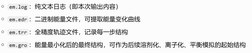
# 程序已自动写入最低能量对应的坐标结构,即输出文件 em.gro
writing lowest energy coordinates.
# 对应就是前面最后一步迭代的结果
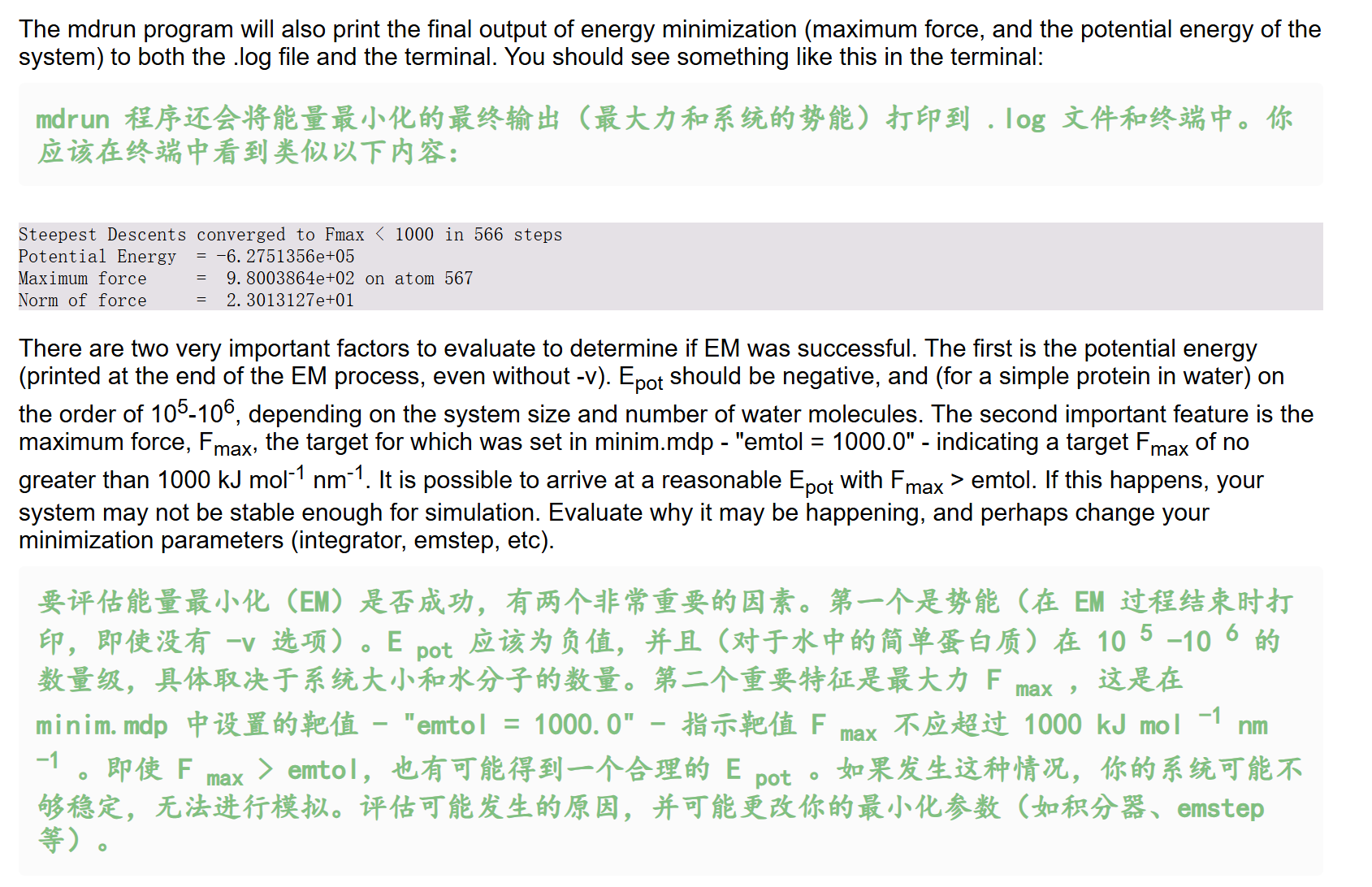
Steepest Descents converged to Fmax < 1000 in 500 steps
Potential Energy = -6.2431850e+05
Maximum force = 8.8014557e+02 on atom 567
# 体系受力范数:23.95 kJ/(mol·nm),整体受力水平极低
Norm of force = 2.3950709e+01
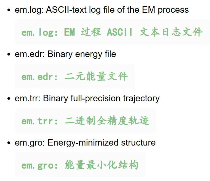
GROMACS reminds you: "If I Were You I Would Give Me a Break" (F. Black)然后生成了4个文件,对应上
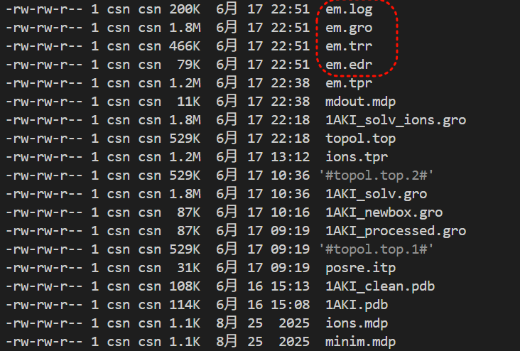
另外比较重要的一点就是评估EM是否成功,看两个指标:
- 结束时的势能
- 结束时的最大力
我们的模拟输出虽然与教程有区别(因为力场文件版本等不能够保持一致),但是基本上都是符合了EM成功的评估
然后就是能量模块分析,使用gmx energy模块
python
gmx energy
gmx help energy
文档指南输出如下
python
Executable:   /home/csn/program/miniconda3/envs/tf-dna-md/bin.AVX2_256/gmx
Data prefix:  /home/csn/program/miniconda3/envs/tf-dna-md
Working dir:  /mnt/sdb/zht/project/tf-dna-md/znf263
Command line:
  gmx help energy

SYNOPSIS

gmx energy [-f [<.edr>]] [-f2 [<.edr>]] [-s [<.tpr>]] [-o [<.xvg>]]
           [-viol [<.xvg>]] [-pairs [<.xvg>]] [-corr [<.xvg>]]
           [-vis [<.xvg>]] [-evisco [<.xvg>]] [-eviscoi [<.xvg>]]
           [-ravg [<.xvg>]] [-odh [<.xvg>]] [-b <time>] [-e <time>] [-[no]w]
           [-xvg <enum>] [-[no]fee] [-fetemp <real>] [-zero <real>]
           [-[no]sum] [-[no]dp] [-nbmin <int>] [-nbmax <int>] [-[no]mutot]
           [-[no]aver] [-nmol <int>] [-[no]fluct_props] [-[no]driftcorr]
           [-[no]fluc] [-[no]orinst] [-[no]ovec] [-einstein_restarts <int>]
           [-einstein_blocks <int>] [-acflen <int>] [-[no]normalize]
           [-P <enum>] [-fitfn <enum>] [-beginfit <real>] [-endfit <real>]

DESCRIPTION

gmx energy extracts energy components from an energy file. The user is
prompted to interactively select the desired energy terms.

Average, RMSD, and drift are calculated with full precision from the
simulation (see printed manual). Drift is calculated by performing a
least-squares fit of the data to a straight line. The reported total drift is
the difference of the fit at the first and last point. An error estimate of
the average is given based on a block averages over 5 blocks using the
full-precision averages. The error estimate can be performed over multiple
block lengths with the options -nbmin and -nbmax. Note that in most cases the
energy files contains averages over all MD steps, or over many more points
than the number of frames in energy file. This makes the gmx energy statistics
output more accurate than the .xvg output. When exact averages are not present
in the energy file, the statistics mentioned above are simply over the single,
per-frame energy values.

The term fluctuation gives the RMSD around the least-squares fit.

Some fluctuation-dependent properties can be calculated provided the correct
energy terms are selected, and that the command line option -fluct_props is
given. The following properties will be computed:

===============================  ===================
Property                         Energy terms needed
===============================  ===================
Heat capacity C_p (NPT sims):    Enthalpy, Temp
Heat capacity C_v (NVT sims):    Etot, Temp
Thermal expansion coeff. (NPT):  Enthalpy, Vol, Temp
Isothermal compressibility:      Vol, Temp
Adiabatic bulk modulus:          Vol, Temp
===============================  ===================

You always need to set the number of molecules -nmol. The C_p/C_v computations
do not include any corrections for quantum effects. Use the gmx dos program if
you need that (and you do).

Option -odh extracts and plots the free energy data (Hamiltoian differences
and/or the Hamiltonian derivative dhdl) from the ener.edr file.

With -fee an estimate is calculated for the free-energy difference with an
ideal gas state:

  Delta A = A(N,V,T) - A_idealgas(N,V,T) = kT
  ln(<exp(U_pot/kT)>)
  Delta G = G(N,p,T) - G_idealgas(N,p,T) = kT
  ln(<exp(U_pot/kT)>)

where k is Boltzmann's constant, T is set by -fetemp and the average is over
the ensemble (or time in a trajectory). Note that this is in principle only
correct when averaging over the whole (Boltzmann) ensemble and using the
potential energy. This also allows for an entropy estimate using:

  Delta S(N,V,T) = S(N,V,T) - S_idealgas(N,V,T) =
  (<U_pot> - Delta A)/T
  Delta S(N,p,T) = S(N,p,T) - S_idealgas(N,p,T) =
  (<U_pot> + pV - Delta G)/T

When a second energy file is specified (-f2), a free energy difference is
calculated:

  dF = -kT
  ln(<exp(-(E_B-E_A) /
  kT)>_A),

where E_A and E_B are the energies from the first and second energy files, and
the average is over the ensemble A. The running average of the free energy
difference is printed to a file specified by -ravg. Note that the energies
must both be calculated from the same trajectory.

For liquids, viscosities can be calculated by integrating the auto-correlation
function of, or by using the Einstein formula for, the off-diagonal pressure
elements. The option -vis turns calculation of the shear and bulk viscosity
through integration of the auto-correlation function. For accurate results,
this requires extremely frequent computation and output of the pressure
tensor. The Einstein formula does not require frequent output and is therefore
more convenient. Note that frequent pressure calculation (nstcalcenergy mdp
parameter) is still needed. Option -evicso gives this shear viscosity estimate
and option -eviscoi the integral. Using one of these two options also triggers
the other. The viscosity is computed from integrals averaged over uniformly
distributed -einstein_restarts starting points, which are sampled over one
block out of -einstein_blocks of the trajectory.

OPTIONS

Options to specify input files:

 -f      [<.edr>]           (ener.edr)
           Energy file
 -f2     [<.edr>]           (ener.edr)       (Opt.)
           Energy file
 -s      [<.tpr>]           (topol.tpr)      (Opt.)
           Portable xdr run input file

Options to specify output files:

 -o      [<.xvg>]           (energy.xvg)
           xvgr/xmgr file
 -viol   [<.xvg>]           (violaver.xvg)   (Opt.)
           xvgr/xmgr file
 -pairs  [<.xvg>]           (pairs.xvg)      (Opt.)
           xvgr/xmgr file
 -corr   [<.xvg>]           (enecorr.xvg)    (Opt.)
           xvgr/xmgr file
 -vis    [<.xvg>]           (visco.xvg)      (Opt.)
           xvgr/xmgr file
 -evisco [<.xvg>]           (evisco.xvg)     (Opt.)
           xvgr/xmgr file
 -eviscoi [<.xvg>]          (eviscoi.xvg)    (Opt.)
           xvgr/xmgr file
 -ravg   [<.xvg>]           (runavgdf.xvg)   (Opt.)
           xvgr/xmgr file
 -odh    [<.xvg>]           (dhdl.xvg)       (Opt.)
           xvgr/xmgr file

Other options:

 -b      <time>             (0)
           Time of first frame to read from trajectory (default unit ps)
 -e      <time>             (0)
           Time of last frame to read from trajectory (default unit ps)
 -[no]w                     (no)
           View output .xvg, .xpm, .eps and .pdb files
 -xvg    <enum>             (xmgrace)
           xvg plot formatting: xmgrace, xmgr, none
 -[no]fee                   (no)
           Do a free energy estimate
 -fetemp <real>             (300)
           Reference temperature for free energy calculation
 -zero   <real>             (0)
           Subtract a zero-point energy
 -[no]sum                   (no)
           Sum the energy terms selected rather than display them all
 -[no]dp                    (no)
           Print energies in high precision
 -nbmin  <int>              (5)
           Minimum number of blocks for error estimate
 -nbmax  <int>              (5)
           Maximum number of blocks for error estimate
 -[no]mutot                 (no)
           Compute the total dipole moment from the components
 -[no]aver                  (no)
           Also print the exact average and rmsd stored in the energy frames
           (only when 1 term is requested)
 -nmol   <int>              (1)
           Number of molecules in your sample: the energies are divided by
           this number
 -[no]fluct_props           (no)
           Compute properties based on energy fluctuations, like heat capacity
 -[no]driftcorr             (no)
           Useful only for calculations of fluctuation properties. The drift
           in the observables will be subtracted before computing the
           fluctuation properties.
 -[no]fluc                  (no)
           Calculate autocorrelation of energy fluctuations rather than energy
           itself
 -[no]orinst                (no)
           Analyse instantaneous orientation data
 -[no]ovec                  (no)
           Also plot the eigenvectors with -oten
 -einstein_restarts <int>   (100)
           Number of restarts for computing the viscosity using the Einstein
           relation
 -einstein_blocks <int>     (4)
           Number of averaging windows for computing the viscosity using the
           Einstein relation
 -acflen <int>              (-1)
           Length of the ACF, default is half the number of frames
 -[no]normalize             (yes)
           Normalize ACF
 -P      <enum>             (0)
           Order of Legendre polynomial for ACF (0 indicates none): 0, 1, 2, 3
 -fitfn  <enum>             (none)
           Fit function: none, exp, aexp, exp_exp, exp5, exp7, exp9
 -beginfit <real>           (0)
           Time where to begin the exponential fit of the correlation function
 -endfit <real>             (-1)
           Time where to end the exponential fit of the correlation function,
           -1 is until the end

GROMACS reminds you: "It's Unacceptable That Chocolate Makes You Fat" (MI 3)
gmx energy 是 GROMACS 分子动力学模拟后最核心的热力学分析工具 ,专门用于读取模拟生成的二进制 .edr 能量文件,提取各类能量/物理量时序数据,计算统计特征与高级热力学性质,输出可直接绘图的 .xvg 格式文件,是模拟结果验证、热力学性质计算的必备工具。
一、核心功能与计算原理
1. 基础能量提取与统计分析
这是该工具最常用的基础功能:
- 交互式选量 :运行后会列出
.edr文件中所有可用的能量项(如势能、动能、总能量、温度、压力、库仑能、范德华能等),用户可通过编号选择一个或多个量进行提取。 - 核心统计量 :自动对选中的物理量计算以下指标,且统计精度高于输出的
.xvg文件(.edr存储了全模拟步长的累计平均,.xvg仅为帧采样数据):- 平均值:全时间段的算术平均
- RMSD(均方根偏差):数据相对于平均值的波动幅度
- 漂移(Drift):通过最小二乘法将数据拟合为直线,取首尾点的差值,反映物理量随时间的整体漂移趋势
- 误差估计 :基于块平均法(默认分为5块)计算平均值的标准误差,可通过参数调整块数范围
2. 高级:涨落热力学性质计算
开启 -fluct_props 参数后,可基于统计力学的涨落公式,从能量、温度、体积的波动中计算宏观热力学响应函数,必须搭配 -nmol 参数指定体系分子数。各性质与所需对应项、适用系综如下:
| 热力学性质 | 所需选中的能量项 | 适用模拟系综 |
|---|---|---|
| 定压热容 (C_p) | 焓(Enthalpy)+ 温度(Temp) | NPT 等温等压系综 |
| 定容热容 (C_v) | 总能量(Etot)+ 温度(Temp) | NVT 正则系综 |
| 热膨胀系数 | 焓 + 体积(Vol)+ 温度 | NPT 系综 |
| 等温压缩系数 | 体积 + 温度 | NPT 系综 |
| 绝热体积模量 | 体积 + 温度 | NPT 系综 |
注意:该计算不包含量子效应修正 ,若需要高精度量子修正结果,需使用
gmx dos工具。
3. 高级:自由能相关计算
工具支持三类自由能分析场景:
- 理想气体参考自由能差(
-fee) :
基于玻尔兹曼平均公式,计算当前体系与相同条件下理想气体的亥姆霍兹自由能差 (Delta A) 和吉布斯自由能差 (Delta G),还可进一步推导熵差。参考温度由-fetemp设置,默认300K。 - 自由能模拟数据提取(
-odh) :
提取 FEP/热力学积分模拟中的哈密顿差、哈密顿导数(dh/dl)数据,用于后续自由能计算。 - 双轨迹自由能差(
-f2) :
输入两个能量文件(来自同一条轨迹的不同哈密顿),通过指数平均公式计算两个状态的自由能差;搭配-ravg可输出自由能差的滑动平均曲线。
4. 高级:粘度计算
针对液体体系,支持两种粘度计算方式:
- 压力张量自相关法(
-vis) :
通过积分压力张量非对角元的自相关函数计算剪切粘度和体积粘度。对模拟设置要求极高,需要极高频率的压力张量输出(远高于常规能量输出频率),否则结果误差极大。 - 爱因斯坦公式法(
-evisco** /-eviscoi)**:
基于爱因斯坦关系计算粘度,对输出频率要求低,使用更便捷,是常规模拟的推荐方案。两个参数分别输出粘度估计值和积分曲线,开启其中一个会自动触发另一个。-einstein_restarts:设置计算的起点数量,默认100,数量越多结果越稳定-einstein_blocks:设置平均的窗口数,默认4
二、输入与输出文件说明
1. 输入文件
| ##### 参数 | ##### 默认文件名 | ##### 必要性 | ##### 说明 |
|---|---|---|---|
##### -f |
##### ener.edr |
##### 必需 | ##### 主能量文件,存储模拟过程中所有能量、温度、压力等时序数据 |
##### -f2 |
##### ener.edr |
##### 可选 | ##### 第二个能量文件,仅用于双轨迹自由能差计算 |
##### -s |
##### topol.tpr |
##### 可选 | ##### 模拟运行输入文件,部分高级计算需要读取拓扑信息 |
2. 输出文件
| 参数 | 默认文件名 | 说明 |
|---|---|---|
-o |
energy.xvg |
主输出文件,存储选中能量项的时序数据,可直接用 xmgrace、Python 绘图 |
-viol |
violaver.xvg |
约束违反的平均数据,仅当模拟设置了约束时可用 |
-pairs |
pairs.xvg |
原子对相互作用的能量数据 |
-corr |
enecorr.xvg |
能量自相关函数数据 |
-vis |
visco.xvg |
自相关法计算的粘度结果 |
-evisco |
evisco.xvg |
爱因斯坦法计算的粘度结果 |
-eviscoi |
eviscoi.xvg |
爱因斯坦法粘度的积分曲线 |
-ravg |
runavgdf.xvg |
自由能差的滑动平均曲线 |
-odh |
dhdl.xvg |
自由能模拟的哈密顿导数(dhdl)数据 |
三、核心常用参数分类解析
1. 时间范围控制
-b <时间>:设置读取的起始时间,单位 ps,默认从0开始-e <时间>:设置读取的结束时间,单位 ps,默认0表示读取到最后一帧
常用于跳过模拟前期的平衡阶段,仅对稳定区间的数据进行统计。
2. 输出与精度控制
-[no]w:是否自动打开 xmgrace 查看输出图像,默认关闭(-now)-xvg <格式>:设置.xvg文件的格式,可选xmgrace(默认)、xmgr、none(无格式纯数据)-[no]dp:是否以双精度高精度输出能量数值,默认关闭-[no]sum:是否将所有选中的能量项求和后输出,而非分别输出,默认关闭
3. 统计与误差控制
-nbmin <整数>、-nbmax <整数>:设置块平均法的最小/最大块数,默认均为5。调整块数可检验误差估计的可靠性。-[no]aver:是否额外输出能量文件中存储的精确平均和 RMSD,仅当只选中1个能量项时可用,默认关闭。
4. 涨落性质专属参数
-[no]fluct_props:开启涨落热力学性质计算,默认关闭-nmol <整数>:体系的分子数,计算涨落性质必须设置,默认1-[no]driftcorr:计算涨落前,先扣除数据的线性漂移趋势,提升涨落计算准确性,默认关闭
5. 自相关与拟合参数
-acflen <整数>:自相关函数的长度,默认-1表示取总帧数的一半-[no]normalize:是否对自相关函数做归一化处理,默认开启-P <阶数>:自相关计算使用的勒让德多项式阶数,0表示不使用-fitfn <函数>:对自相关函数的拟合函数,可选none(默认)、exp(单指数)、aexp、exp_exp(双指数)等-beginfit <时间>、-endfit <时间>:设置拟合的时间区间,-endfit为-1表示拟合到末尾
四、核心重点提炼
- 工具定位 :GROMACS 标准热力学分析工具,专门处理二进制
.edr能量文件,是模拟收敛性验证、热力学性质计算的核心入口。 - 基础能力(最常用) :
- 交互式提取势能、温度、压力等任意能量项,输出时序数据
- 自动计算平均值、波动幅度、整体漂移、统计误差,且终端统计结果精度高于
.xvg文件
- 高级能力 :
- 基于涨落公式计算热容、热膨胀系数、压缩系数等宏观热力学量,需匹配对应系综,且必须设置
-nmol - 支持三类自由能分析:理想气体参考差、FEP 数据提取、双轨迹自由能差
- 提供两种粘度计算方案,常规模拟优先推荐爱因斯坦法
- 基于涨落公式计算热容、热膨胀系数、压缩系数等宏观热力学量,需匹配对应系综,且必须设置
- 注意事项 :
- 涨落性质计算无量子修正,高精度需求需搭配
gmx dos - 自相关法粘度对压力输出频率要求极高,常规模拟不推荐使用
- 涨落性质计算无量子修正,高精度需求需搭配
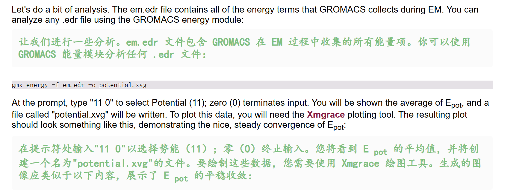
然后我们的命令如下
python
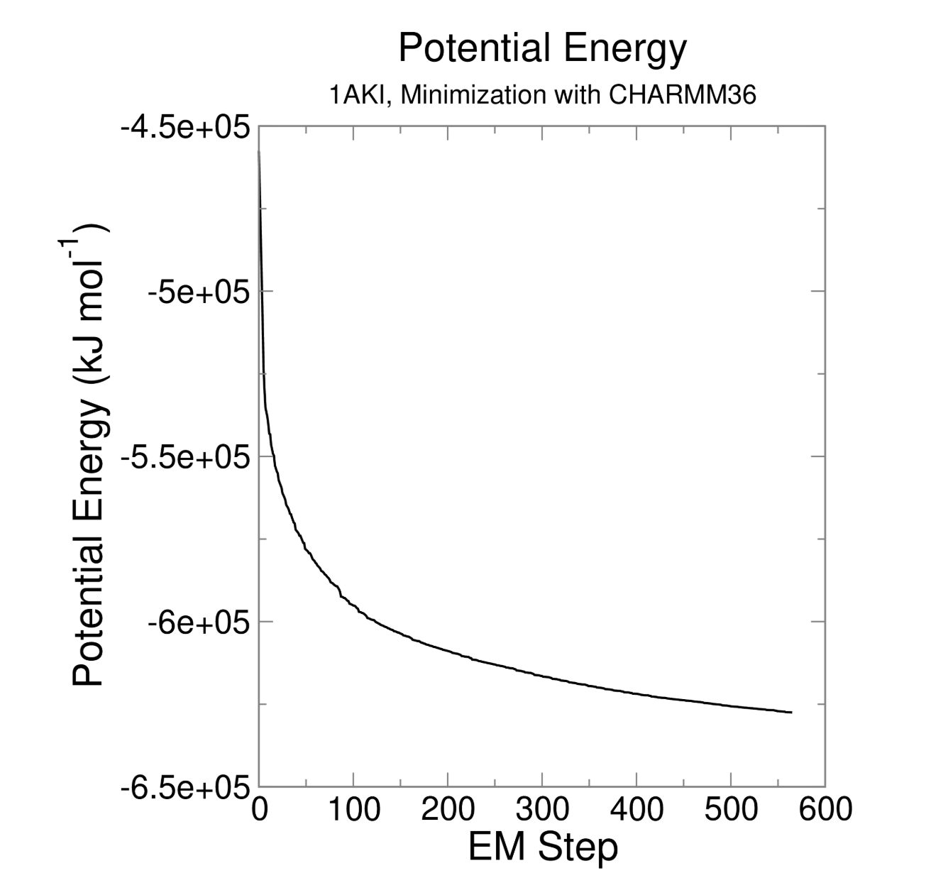
gmx energy -f em.edr -o potential.xvg这个命令很简单,就是读取能量最小化输出的 em.edr 二进制能量文件,提取势能(Potential)随迭代步数的变化曲线,输出文本绘图文件 potential.xvg,用于可视化查看 EM 全过程势能下降是否收敛、结构优化是否正常
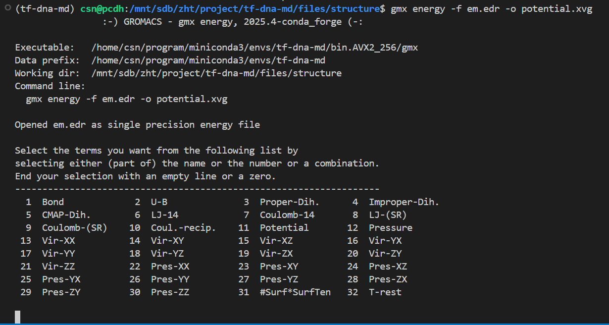
这也是一个交互式的选择,因为教程中我们目前只看势能,所以选择11,然后输入0作为终止符
输出结果如下
整体日志如下:
python
Command line:
gmx energy -f em.edr -o potential.xvg
Opened em.edr as single precision energy file
Select the terms you want from the following list by
selecting either (part of) the name or the number or a combination.
End your selection with an empty line or a zero.
-------------------------------------------------------------------
1 Bond 2 U-B 3 Proper-Dih. 4 Improper-Dih.
5 CMAP-Dih. 6 LJ-14 7 Coulomb-14 8 LJ-(SR)
9 Coulomb-(SR) 10 Coul.-recip. 11 Potential 12 Pressure
13 Vir-XX 14 Vir-XY 15 Vir-XZ 16 Vir-YX
17 Vir-YY 18 Vir-YZ 19 Vir-ZX 20 Vir-ZY
21 Vir-ZZ 22 Pres-XX 23 Pres-XY 24 Pres-XZ
25 Pres-YX 26 Pres-YY 27 Pres-YZ 28 Pres-ZX
29 Pres-ZY 30 Pres-ZZ 31 #Surf*SurfTen 32 T-rest
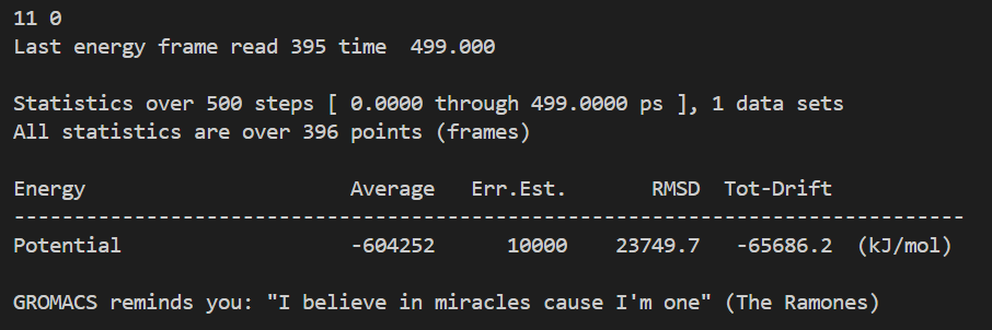
11 0
# EM 一共跑了 500 步,时间轴单位 ps,区间 0 ~ 499 ps
# 总共读取到 396 个有效采样帧(不是每一步都输出能量,mdp 里 nstenergy 控制输出间隔,所以帧数少于总步数)
Last energy frame read 395 time 499.000
# 只提取了 1 组物理量:势能 Potential
Statistics over 500 steps [ 0.0000 through 499.0000 ps ], 1 data sets
All statistics are over 396 points (frames)
# ⚠️ 核心统计结果
Energy Average Err.Est. RMSD Tot-Drift
-------------------------------------------------------------------------------
Potential -604252 10000 23749.7 -65686.2 (kJ/mol)
# Average 平均值:-604252 kJ/mol
# 整个 EM 0~500 步全部采样点的势能算术平均值
# 初始势能约 - 45.6 万,最终收敛到 - 62.4 万,均值落在两者中间,符合持续下降趋势
# Err.Est. 误差估计:10000 kJ/mol
# 采用块平均法计算均值的统计误差,数值偏大是因为 EM 前期势能剧烈下降,数据波动极大;平衡模拟的误差会小很多
# RMSD 均方根波动:23749.7 kJ/mol
# 所有势能数据相对平均值的波动幅度,数值大代表 EM 全过程能量变化剧烈,属于能量最小化正常现象(平衡 NVT/NPT 阶段 RMSD 会显著变小)
# Tot-Drift 总漂移:-65686.2 kJ/mol
# 对势能随时间做最小二乘线性拟合,末尾值 - 初始值 = -65686.2
# 负数代表势能整体持续降低,完美证明 EM 优化有效,体系不断释放不合理内能这一步只有1个输出文件
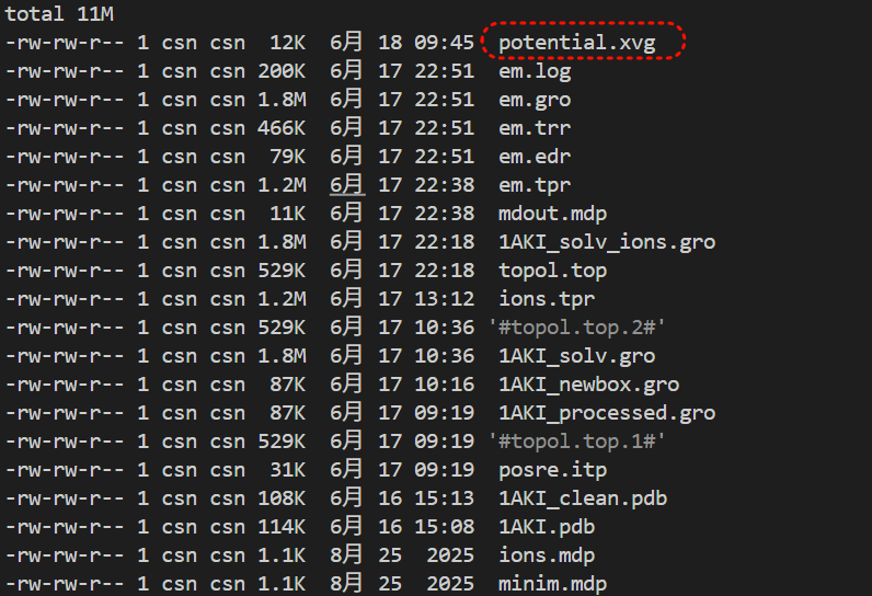
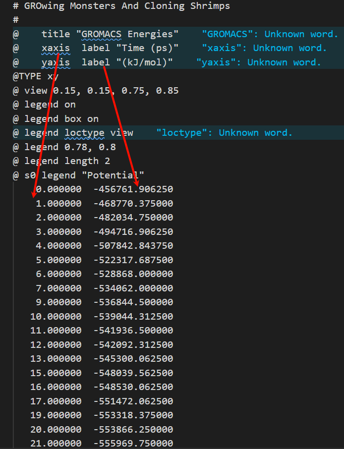
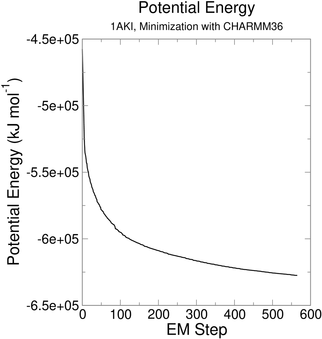
这个文本文件其实就是二维坐标图

教程中是使用了一个绘图工具Xmgrace,
https://plasma-gate.weizmann.ac.il/Grace/
这里给出几个选择,都可以用于绘制这个xvg文件,主要是集中于python库
- Matplotlib + Numpy:跳过开头的注释行即可
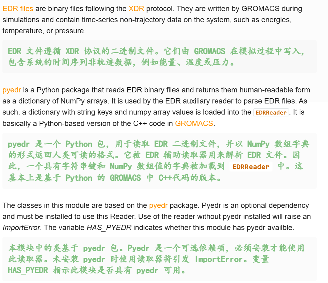
- MDAnalysis库:核心依赖是pyedr
仓库参考:https://github.com/MDAnalysis/mdanalysis
参考:https://userguide.mdanalysis.org/stable/formats/auxiliary.html
以及https://docs.mdanalysis.org/2.8.0/documentation_pages/auxiliary/EDR.html
我们需要查看一下加载进去的这个文件有什么属性
python
import MDAnalysis as mda
aux = mda.auxiliary.EDR.EDRReader("/mnt/sdb/zht/project/tf-dna-md/files/structure/em.edr")
# 查看属性
aux.terms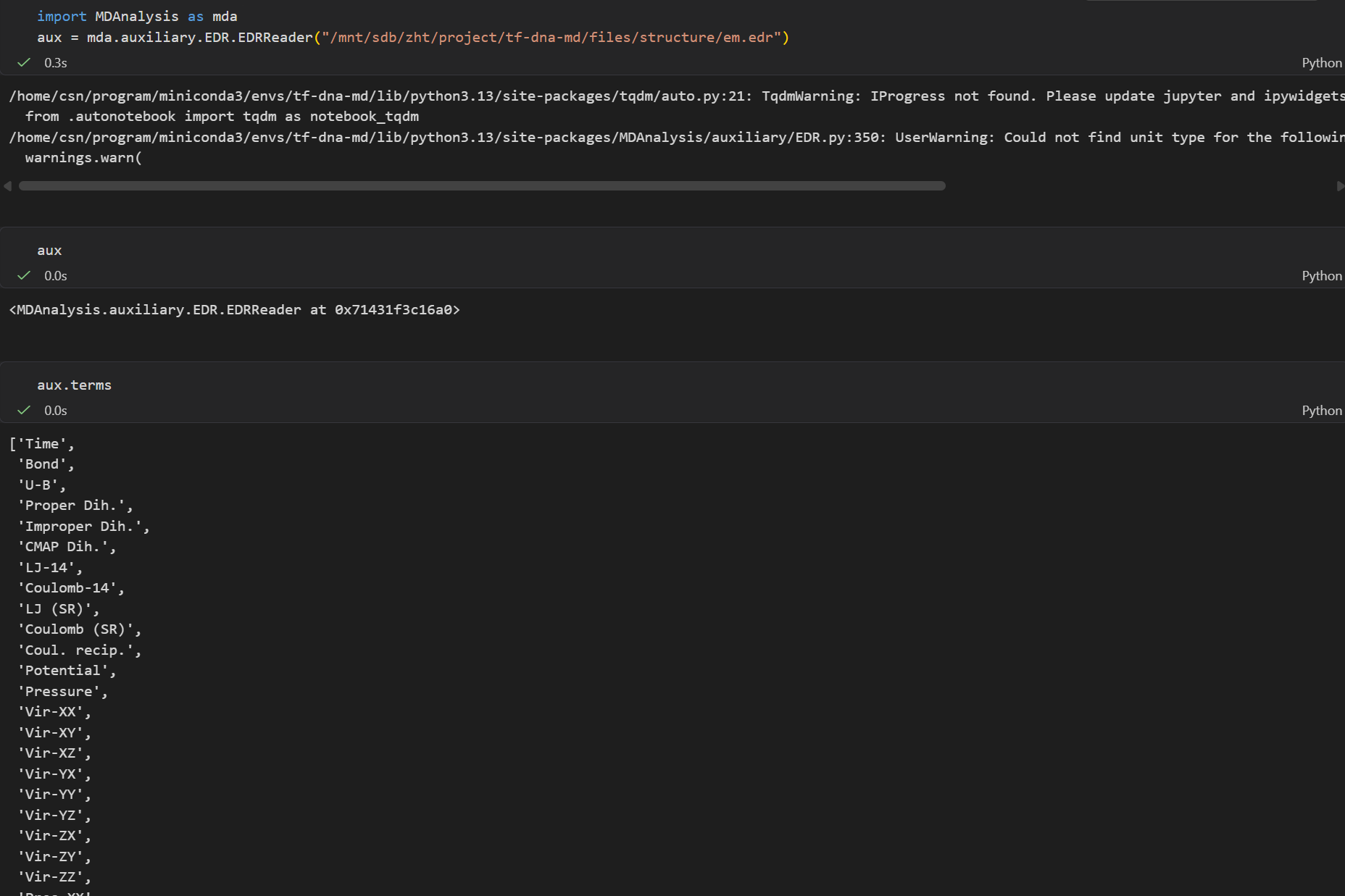
我们就选择这里的势能项,
python
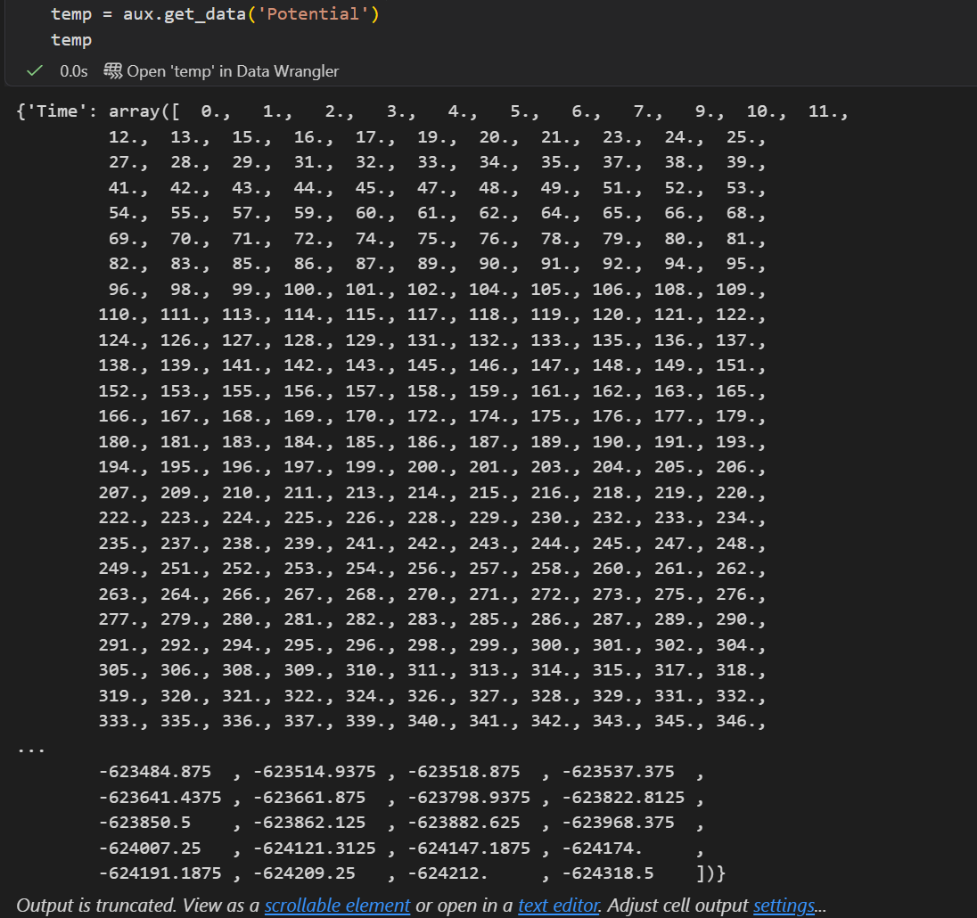
temp = aux.get_data('Potential')
temp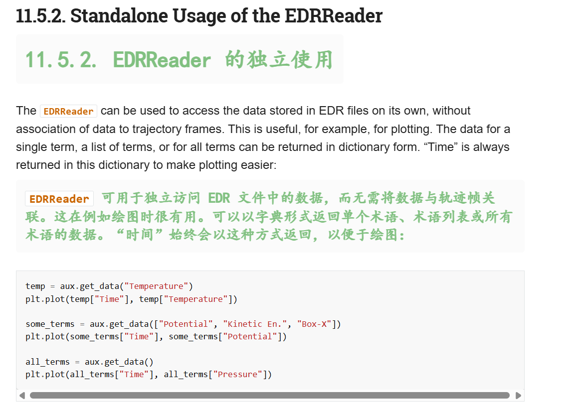
看着像是有两个键值对的一维数组
有数据了绘图就很简单了
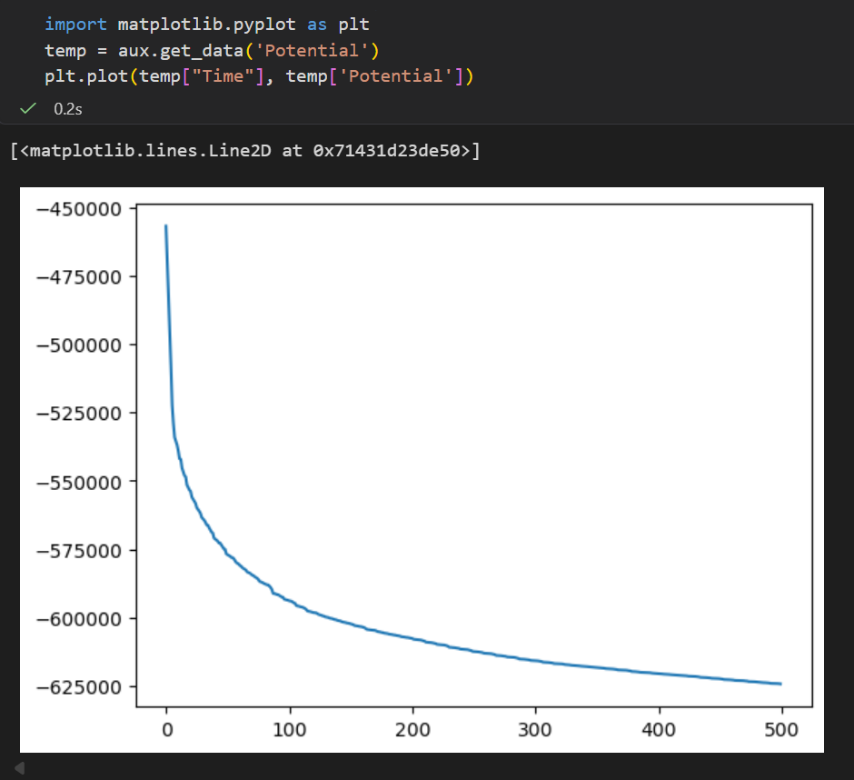
python
import matplotlib.pyplot as plt
temp = aux.get_data('Potential')
plt.plot(temp["Time"], temp['Potential'])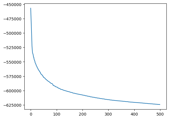
另外也可以参考一下:https://github.com/MDAnalysis/panedr
- 还有一些第三方的xvg绘图工具:
参考:https://github.com/TheBiomics/GMXvg
https://github.com/JoaoRodrigues/gmx-tools
总而言之,我们可以进入下一步了

6,Equilibration
能量最小化只是确保我们有一个合理的初始结构,而平衡则是下一步所需要的
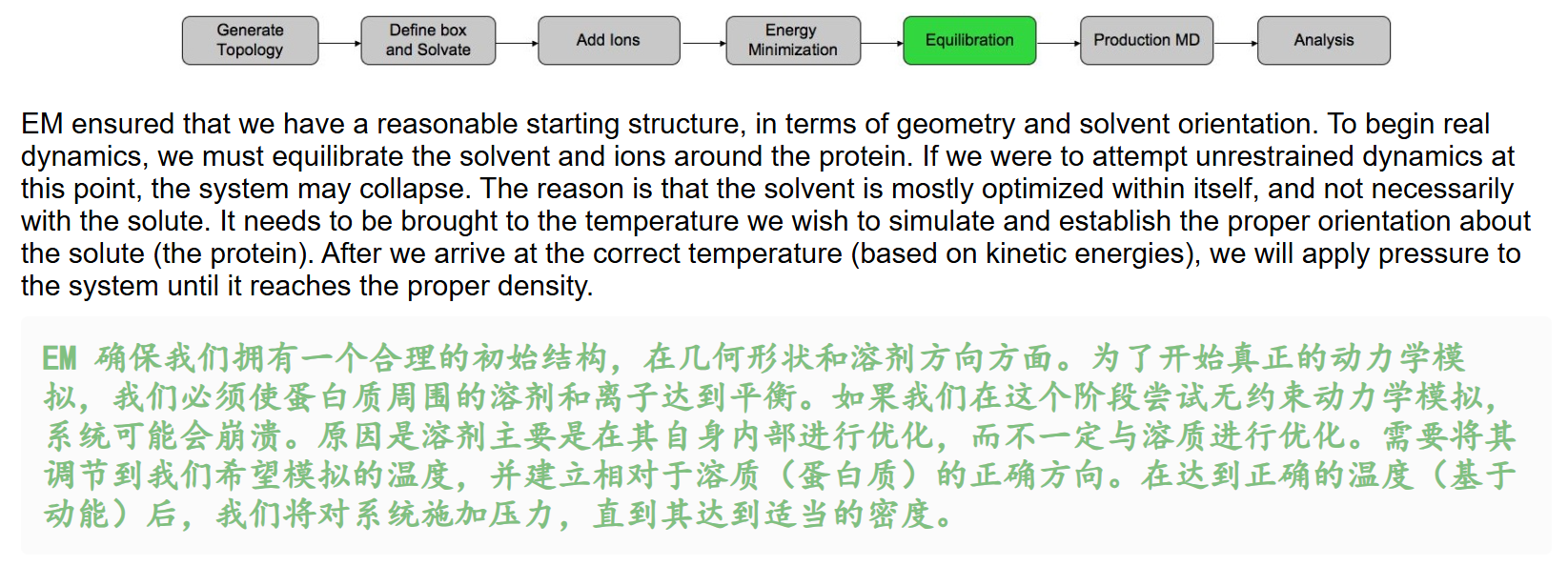
总得来说:
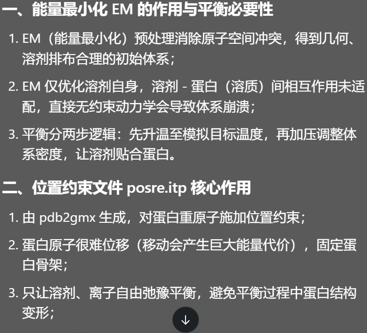
- EM是针对溶剂优化,溶剂-溶质本身还没有优化
- 平衡分两步,先调温,再加压
第1阶段平衡:NVT
NVT 恒温恒容平衡(粒子数 N、体积 V、温度 T 不变),目标:让体系温度稳定在设定值(298K),时长常规 50--100 ps,本例跑 100 ps。
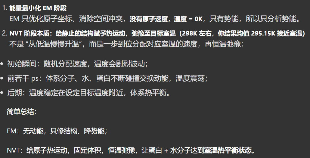
简单来说就是,我们先设置成目标温度(室温),然后在这个温度下慢慢弛豫,就是拿到我们目标温度恒温定容平衡模拟结果。
同样的,我们需要运行一次常规模拟,
基本路数我们都已经门清了,
配置mdp文件,跑grompp;得到tpr文件之后跑mdrun
配置mdp文件我们从教程中获取,http://www.mdtutorials.com/gmx/lysozyme/Files/nvt.mdp
这个文件的配置就比较长了
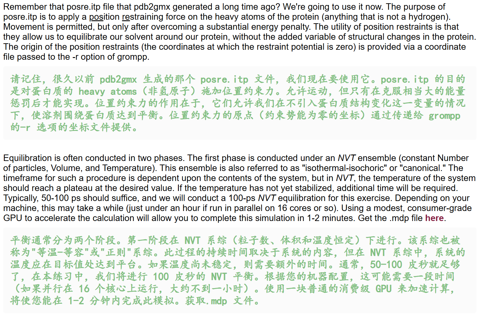
python
title                   = OPLS Lysozyme NVT equilibration
define                  = -DPOSRES  ; position restrain the protein
; Run parameters
integrator              = md        ; leap-frog integrator
nsteps                  = 50000     ; 2 * 50000 = 100 ps
dt                      = 0.002     ; 2 fs
; Output control
nstxout                 = 2500      ; save coordinates every 5.0 ps
nstvout                 = 2500      ; save velocities every 5.0 ps
nstenergy               = 2500      ; save energies every 5.0 ps
nstlog                  = 2500      ; update log file every 5.0 ps
; Bond parameters
continuation            = no        ; first dynamics run
constraint_algorithm    = lincs     ; holonomic constraints
constraints             = h-bonds   ; bonds involving H are constrained
lincs_iter              = 1         ; accuracy of LINCS
lincs_order             = 4         ; also related to accuracy
; Nonbonded settings
cutoff-scheme           = Verlet    ; Buffered neighbor searching
ns_type                 = grid      ; search neighboring grid cells
nstlist                 = 10        ; 20 fs, largely irrelevant with Verlet
; vdW
rvdw                    = 1.2       ; short-range van der Waals cutoff (in nm)
rvdw-switch             = 1.0
vdw-modifier            = force-switch
DispCorr                = No        ; per CHARMM FF convention
; Electrostatics
rcoulomb                = 1.2       ; short-range electrostatic cutoff (in nm)
coulombtype             = PME       ; Particle Mesh Ewald for long-range electrostatics
pme_order               = 4         ; cubic interpolation
fourierspacing          = 0.16      ; grid spacing for FFT
; Temperature coupling is on
tcoupl                  = V-rescale ; stochastic Bussi thermostat
tc-grps                 = System
tau_t                   = 1.0       ; value of tau (ps)
ref_t                   = 298       ; temperature (K)
; Pressure coupling is off
pcoupl                  = no        ; no pressure coupling in NVT
; Periodic boundary conditions
pbc                     = xyz       ; 3-D PBC
; Velocity generation
gen_vel                 = yes       ; assign velocities from Maxwell distribution
gen_temp                = 298       ; temperature for Maxwell distribution
gen_seed                = -1        ; generate a random seed
我添加中文笔记如下
python
; ==============================================================================
; 【NVT平衡模拟说明】
; EM能量最小化仅优化体系几何与溶剂自身排布,溶剂并未与蛋白溶质协同平衡;
; 若直接放开约束跑无限制动力学,溶剂剧烈运动会造成体系结构崩溃。
; NVT阶段目标:固定盒子体积、约束蛋白骨架,仅平衡溶剂/离子,将体系升温至298K,
; 使溶剂在蛋白周围形成合理排布;待温度稳定后,再进入NPT阶段控压调整体系密度。
; 本文件启用-DPOSRES,调用pdb2gmx生成的posre.itp,对蛋白重原子施加位置约束;
; 蛋白偏离参考坐标会产生能量惩罚,大幅限制蛋白构象变动,仅让溶剂自由弛豫平衡。
; 约束参考坐标由grompp -r em.gro 指定,以能量最小化后的稳定结构为基准。
; 平衡分两步:NVT(定容定温)→ NPT(定压调密度);本模拟总时长100 ps。
; ==============================================================================
title                   = OPLS Lysozyme NVT equilibration
define                  = -DPOSRES  ; 开启蛋白重原子位置约束,读取posre.itp
; Run parameters 动力学核心参数
integrator              = md        ; leap-frog蛙跳积分器,标准分子动力学算法
nsteps                  = 50000     ; 总步数50000,dt=2fs,总模拟时长50000*0.002=100 ps
dt                      = 0.002     ; 积分步长2 fs,约束氢键后可使用该大步长
; Output control 输出记录频率,每2500步=5 ps输出一次轨迹、能量、日志
nstxout                 = 2500      ; 输出原子坐标轨迹
nstvout                 = 2500      ; 输出原子速度
nstenergy               = 2500      ; 输出能量至edr文件,用于后续温度/势能分析
nstlog                  = 2500      ; 更新文本日志log文件
; Bond parameters 化学键约束设置
continuation            = no        ; 全新动力学模拟,不接续之前轨迹
constraint_algorithm    = lincs     ; LINCS约束算法,处理含氢化学键
constraints             = h-bonds   ; 约束所有H参与的化学键,允许2fs步长
lincs_iter              = 1         ; LINCS迭代精度
lincs_order             = 4         ; LINCS高阶修正精度
; Nonbonded settings 非键相互作用(范德华),适配OPLS/CHARMM力场
cutoff-scheme           = Verlet    ; Verlet缓冲邻域搜索,计算效率更高
ns_type                 = grid      ; 网格划分搜索邻近原子
nstlist                 = 10        ; 邻域列表更新间隔,Verlet方案下影响很小
rvdw                    = 1.2       ; 范德华短程截断距离1.2 nm
rvdw-switch             = 1.0       ; 1.0 nm处开始平滑切换范德华势能至0
vdw-modifier            = force-switch ; 力平滑切换,避免截断处受力突变
DispCorr                = No        ; 关闭色散能量修正,遵循OPLS/CHARMM规范
; Electrostatics 长程静电作用 PME算法
rcoulomb                = 1.2       ; 短程静电截断1.2 nm
coulombtype             = PME       ; PME网格埃瓦尔德,处理长程静电相互作用
pme_order               = 4         ; 4次插值PME网格
fourierspacing          = 0.16      ; FFT傅里叶网格间距0.16 nm
; Temperature coupling NVT核心:V-rescale控温
tcoupl                  = V-rescale ; Bussi随机速度标度控温,温度平衡稳定无伪影
tc-grps                 = System    ; 整个体系作为单一控温组
tau_t                   = 1.0       ; 温度耦合弛豫时间1 ps
ref_t                   = 298       ; 目标平衡温度298 K
; Pressure coupling NVT特征:关闭控压,盒子体积固定不变
pcoupl                  = no        ; NVT系综无压力耦合,体积恒定
; Periodic boundary conditions 三维周期性边界模拟溶液环境
pbc                     = xyz       ; x/y/z三个方向均开启周期性边界
; Velocity generation 初始化原子速度
gen_vel                 = yes       ; 基于麦克斯韦分布随机分配初始速度
gen_temp                = 298       ; 速度分布对应温度298 K
gen_seed                = -1        ; 随机种子自动生成,每次模拟初速度不同
我们的命令如下
python
# NVT模拟,先获取tpr
gmx grompp -f nvt.mdp -c em.gro -r em.gro -p topol.top -o nvt.tpr

# 开始模拟
gmx mdrun -deffnm nvt
-c 是现在原子在哪;-r 是原子被强制不许远离的模板位置。

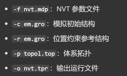
先获取tpr输出日志如下
python
Executable:   /home/csn/program/miniconda3/envs/tf-dna-md/bin.AVX2_256/gmx
Data prefix:  /home/csn/program/miniconda3/envs/tf-dna-md
Working dir:  /mnt/sdb/zht/project/tf-dna-md/files/structure
Command line:
  gmx grompp -f nvt.mdp -c em.gro -r em.gro -p topol.top -o nvt.tpr

Ignoring obsolete mdp entry 'title'
Ignoring obsolete mdp entry 'ns_type'

# 1️⃣随机种子初始化
# 生成两个独立随机种子:
# LD 种子:用于控温、随机动力学;
Setting the LD random seed to -31457857

# 2️⃣非键、1-4 相互作用参数加载
# 成功加载范德华、静电非键参数
Generated 169542 of the 169653 non-bonded parameter combinations
# 1-4 相互作用缩放系数 fudge=1,匹配选用的 OPLS 力场
Generating 1-4 interactions: fudge = 1
# 绝大多数原子对参数匹配成功,无报错,拓扑参数正常
Generated 118878 of the 169653 1-4 parameter combinations

# 3️⃣蛋白、水分子、氯离子体系全部开启氢键约束,氢原子运动被固定,允许使用 2 fs 时间步长,和 mdp 设置完全一致
Excluding 3 bonded neighbours molecule type 'Protein_chain_A'

turning H bonds into constraints...

Excluding 2 bonded neighbours molecule type 'SOL'

turning H bonds into constraints...

Excluding 3 bonded neighbours molecule type 'CL'

turning H bonds into constraints...

# 1️⃣gen_seed:用于生成 298K 麦克斯韦速度分布
# 对应前面的生成两个随机种子
Setting gen_seed to -42141889
# 都符合mdp设置中gen_vel=yes gen_temp=298 的设置,会给所有原子分配符合室温的初始速度
Velocities were taken from a Maxwell distribution at 298 K

# 4️⃣体系组分统计
# 体系组成清晰:129 个蛋白残基 + 大量水 + 8 个氯离子;
# 整体作为单一控温组System,总自由度 80476,V-rescale 控温正常生效。
Analysing residue names:
There are:   129    Protein residues
There are: 12589      Water residues
There are:     8        Ion residues
Analysing Protein...
Number of degrees of freedom in T-Coupling group System is 80476.00

# 5️⃣邻域列表 Verlet 参数计
# 排除原子间最大距离 0.441 nm,无近距离原子重叠问题
# Verlet 缓冲区间自动计算,邻域截断 rlist=1.2 nm,和范德华截断 rvdw=1.2 nm 匹配
# 实际运行时 mdrun 会自动重新适配邻域列表,无需手动调整
The largest distance between excluded atoms is 0.441 nm between atom 1156 and 1405

Determining Verlet buffer for a tolerance of 0.005 kJ/mol/ps at 298 K
Calculated rlist for 1x1 atom pair-list as 1.234 nm, buffer size 0.034 nm
Set rlist, assuming 4x4 atom pair-list, to 1.200 nm, buffer size 0.000 nm

Note that mdrun will redetermine rlist based on the actual pair-list setup

# 开启位置约束时,程序会移除体系质心运动,理论上可能产生微小数值伪影;但大分子 NVT 平衡阶段影响几乎可以忽略,行业标准操作,无需修改任何参数。
NOTE 1 [file nvt.mdp]:
  Removing center of mass motion in the presence of position restraints
  might cause artifacts. When you are using position restraints to
  equilibrate a macro-molecule, the artifacts are usually negligible.

# 6️⃣ PME 长程静电网格
Calculating fourier grid dimensions for X Y Z
# PME 傅里叶网格 48×48×48,网格间距~0.154 nm,接近设置的 fourierspacing=0.16,自动适配盒子尺寸
Using a fourier grid of 48x48x48, spacing 0.154 0.154 0.154
# PME 网格计算负载仅占总计算量 15%,算力开销小,模拟速度有保障
Estimate for the relative computational load of the PME mesh part: 0.15

This run will generate roughly 22 Mb of data

# 见前面note1
There was 1 NOTE

GROMACS reminds you: "If you're doing I/O, you're doing it wrong!" (Cannada "Drew" Lewis)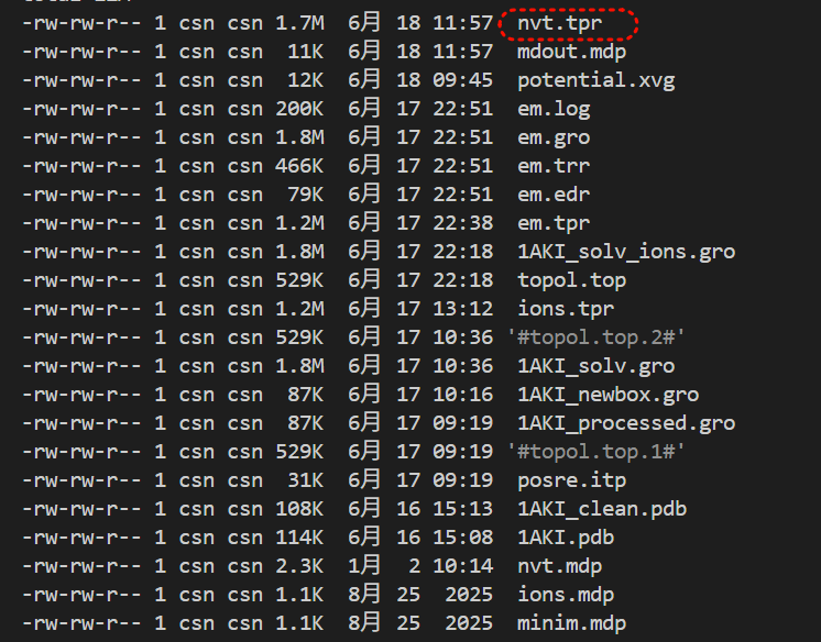
我们再开始模拟(gmx mdrun -deffnm nvt),
输出日志如下:
python
Executable:   /home/csn/program/miniconda3/envs/tf-dna-md/bin.AVX2_256/gmx
Data prefix:  /home/csn/program/miniconda3/envs/tf-dna-md
Working dir:  /mnt/sdb/zht/project/tf-dna-md/files/structure
Command line:
  gmx mdrun -deffnm nvt

Compiled SIMD is AVX2_256, but AVX_512 might be faster (see log).
The current CPU can measure timings more accurately than the code in
gmx mdrun was configured to use. This might affect your simulation
speed as accurate timings are needed for load-balancing.
Please consider rebuilding gmx mdrun with the GMX_USE_RDTSCP=ON CMake option.
Reading file nvt.tpr, VERSION 2025.4-conda_forge (single precision)
Changing nstlist from 10 to 80, rlist from 1.2 to 1.322

# 总 CPU 核心占用:32×1 = 32 核纯 MPI,无多线程并行
Using 32 MPI threads
Using 1 OpenMP thread per tMPI thread

starting mdrun 'LYSOZYME in water'
50000 steps,    100.0 ps.

Writing final coordinates.

# ⚠️ 关键负载失衡报告(核心问题)
Dynamic load balancing report:
 DLB got disabled because it was unsuitable to use.
 Average load imbalance: 39.4%.
 The balanceable part of the MD step is 52%, load imbalance is computed from this.
# 域分解 DD 负载失衡(损失 20.7% CPU 时间)
# DLB动态负载均衡直接被禁用(体系不适合开DLB)
# 溶菌酶蛋白是致密大分子,盒子内粒子分布极度不均匀;32 个 MPI 域均分盒子后,部分域全是水分子、部分域塞满蛋白原子,算力差距巨大,动态负载均衡 DLB 无法修复直接关闭。
 Part of the total run time spent waiting due to load imbalance: 20.7%.
 Average PME mesh/force load: 0.630
# PP/PME 算力不匹配(额外损失 8.2% 性能)
# PME网格/力负载均值0.630,PME进程工作量远少于PP实空间进程
# PME 负责长程静电,PP 负责短程范德华 + 键合作用;现在 PME 进程太闲,PP 忙不过来
 Part of the total run time spent waiting due to PP/PME imbalance: 8.2 %

NOTE: 20.7 % of the available CPU time was lost due to load imbalance
      in the domain decomposition.
      You can consider manually changing the decomposition (option -dd);
      e.g. by using fewer domains along the box dimension in which there is
      considerable inhomogeneity in the simulated system.
NOTE: 8.2 % performance was lost because the PME ranks
      had less work to do than the PP ranks.
      You might want to decrease the number of PME ranks
      or decrease the cut-off and the grid spacing.


               Core t (s)   Wall t (s)        (%)
       Time:    14520.175      453.756     3200.0
                 (ns/day)    (hour/ns)
Performance:       19.041        1.260

GROMACS reminds you: "Trying is the first step towards failure." (Homer Simpson)
轨迹 / 能量文件完整可用,只是计算效率低,
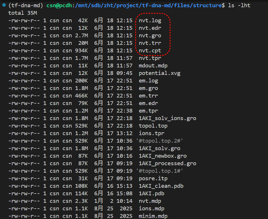
因为我们的目的是控温,所以看看温度变化是关键(就像前面那个能量最小化,能量最关键,所以我们需要看看)。
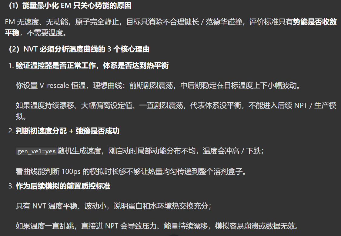
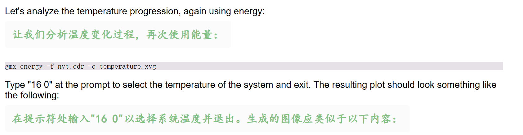
这回我们选择16,也就是温度
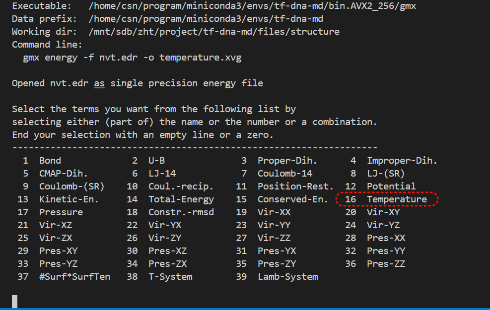
日志粘贴如下
python
Executable:   /home/csn/program/miniconda3/envs/tf-dna-md/bin.AVX2_256/gmx
Data prefix:  /home/csn/program/miniconda3/envs/tf-dna-md
Working dir:  /mnt/sdb/zht/project/tf-dna-md/files/structure
Command line:
  gmx energy -f nvt.edr -o temperature.xvg

Opened nvt.edr as single precision energy file

Select the terms you want from the following list by
selecting either (part of) the name or the number or a combination.
End your selection with an empty line or a zero.
-------------------------------------------------------------------
  1  Bond             2  U-B              3  Proper-Dih.      4  Improper-Dih.
  5  CMAP-Dih.        6  LJ-14            7  Coulomb-14       8  LJ-(SR)
  9  Coulomb-(SR)    10  Coul.-recip.    11  Position-Rest.  12  Potential
 13  Kinetic-En.     14  Total-Energy    15  Conserved-En.   16  Temperature
 17  Pressure        18  Constr.-rmsd    19  Vir-XX          20  Vir-XY
 21  Vir-XZ          22  Vir-YX          23  Vir-YY          24  Vir-YZ
 25  Vir-ZX          26  Vir-ZY          27  Vir-ZZ          28  Pres-XX
 29  Pres-XY         30  Pres-XZ         31  Pres-YX         32  Pres-YY
 33  Pres-YZ         34  Pres-ZX         35  Pres-ZY         36  Pres-ZZ
 37  #Surf*SurfTen   38  T-System        39  Lamb-System

16 0
Last energy frame read 20 time  100.000

# 总模拟:0~100 ps,50001 步,输出 501 个温度采样点;
Statistics over 50001 steps [ 0.0000 through 100.0000 ps ], 1 data sets
All statistics are over 501 points

# Average 平均值 = 295.152 K
# 接近生理室温 298K,说明温控整体达标,体系平均温度符合预期

# Err.Est. 误差估计 = 3.2 K
# 温度统计标准误差,数值越小代表整体波动越小;3.2 属于中等波动

# RMSD 均方根偏差 = 12.8951 K
# 温度随时间偏离平均值的震荡幅度,12.9K 波动偏大,说明整个 100ps 模拟过程温度起伏明显,体系弛豫还不够充分

# Tot-Drift 总漂移 = 19.4196 K
# 全程从 0ps 到 100ps,温度整体单向偏移幅度高达 19.4K,是比较明显的漂移:
# 意味着模拟初期和末期平均温度有显著差距,100ps NVT 时长不足,体系还没完全热平衡


Energy                      Average   Err.Est.       RMSD  Tot-Drift
-------------------------------------------------------------------------------
Temperature                 295.152        3.2    12.8951    19.4196  (K)

GROMACS reminds you: "What is a Unix or Linux sysadmin's favourite hangout place? Foo Bar." (Anonymous)
同样的,我们可以从xvg图直接去看,
或者想前面那样直接从edr文件中查看。
我们这次试一试直接从前面的Xmgrace
https://plasma-gate.weizmann.ac.il/Grace/
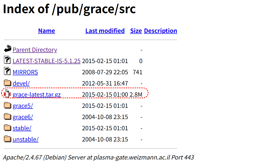
安装解压之后,源码安装细节参考https://plasma-gate.weizmann.ac.il/Grace/doc/UsersGuide.html#ss2.1
python
# 源码树、编译分离
mkdir /tmp/grace-obj
cd /tmp/grace-obj

# 假设我们的软件下载在/mnt/sdb/zht/software/grace-5.1.25
/mnt/sdb/zht/software/grace-5.1.25/ac-tools/shtool  mkshadow /mnt/sdb/zht/software/
grace-5.1.25 .

# 在影子目录里面configure
./configure --enable-grace-home=/opt/grace \
--with-extra-incpath=/usr/local/include:/opt/include \
--with-extra-ldpath=/usr/local/lib:/opt/lib \
--prefix=/usr

# 编译
make -j$(nproc)

# 安装到系统
make install

# 软链接补充
make links
我们此处还是使用edr相关mdanalysis来绘制
python
import MDAnalysis as mda
import matplotlib.pyplot as plt
aux = mda.auxiliary.EDR.EDRReader("/mnt/sdb/zht/project/tf-dna-md/files/structure/nvt.edr")
temp = aux.get_data('Temperature')
plt.plot(temp["Time"], temp['Temperature'])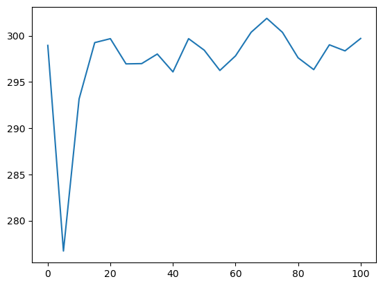
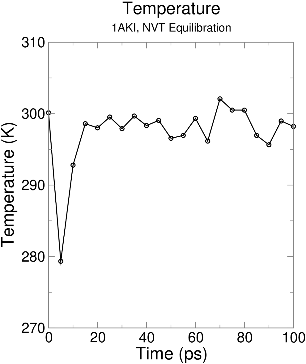
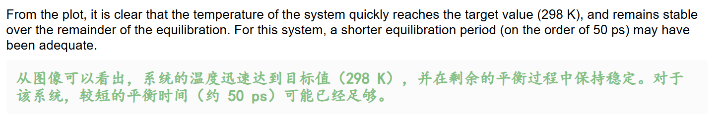
第2阶段平衡:NPT
然后紧接着是第二阶段的平衡,
- 第一阶段:等温等容,NVT(粒子数、体积、温度不变),设置目标温度,进行弛豫(稳定系统温度)
- 第二阶段:等温等压,NPT(粒子数、压强、温度不变),稳定系统压力(同时稳定密度)
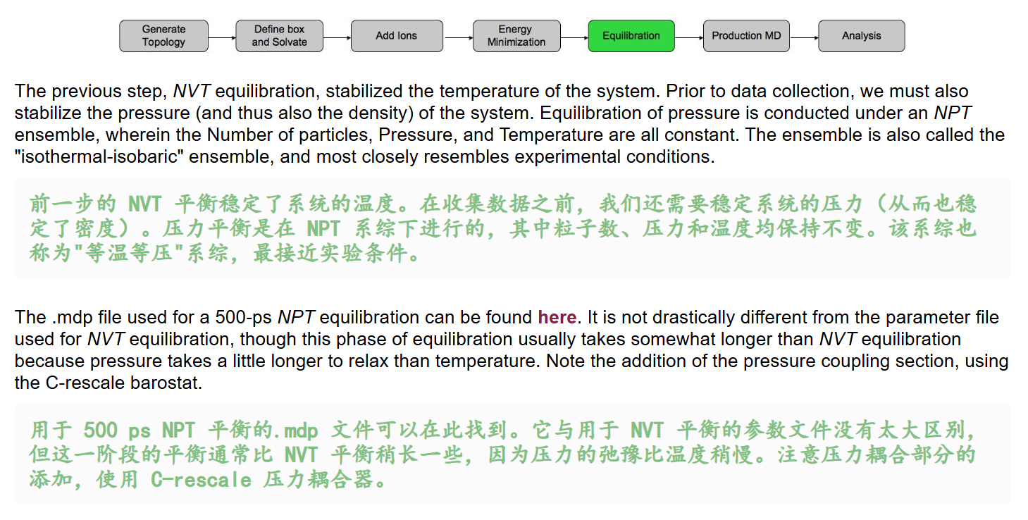
我们同样获取教程中用于NPT平衡的mdp文件,
http://www.mdtutorials.com/gmx/lysozyme/Files/npt.mdp
注释如下
python
;======================== NPT平衡模拟参数 OPLS力场溶菌酶 ========================
; 承接NVT平衡续算,总模拟时长500 ps,蛋白骨架施加位置限制仅弛豫溶剂密度压力
title                   = OPLS Lysozyme NPT equilibration
define                  = -DPOSRES        ; 开启蛋白位置限制,防止盒子缩放扭曲蛋白结构

;======================== 模拟积分与时长设置 ========================
continuation            = yes             ; 续算模式,读取NVT末态坐标与速度,不重新生成速度
integrator              = md              ; leap-frog蛙跳分子动力学积分器
nsteps                  = 250000          ; 总步数25万步,dt=2fs,250000*0.002=500000fs=500ps
dt                      = 0.002           ; 积分步长2 fs,LINCS约束H键支持该步长

;======================== 输出打印控制 每1ps输出一次 ========================
nstxout                 = 500             ; 每500步(1ps)输出原子坐标gro/trr
nstvout                 = 500             ; 每500步输出原子速度
nstenergy               = 500             ; 每500步输出能量、温度、压力、密度至edr
nstlog                  = 500             ; 每500步更新模拟日志log文件

;======================== 化学键约束方案 ========================
constraint_algorithm    = lincs           ; LINCS约束算法,适用于蛋白体系
constraints             = h-bonds         ; 约束所有含氢原子化学键,允许2fs大步长
lincs_iter              = 1               ; LINCS迭代精度
lincs_order             = 4               ; LINCS展开阶数,提升约束精度

;======================== 范德华非键相互作用 ========================
cutoff-scheme           = Verlet          ; Verlet缓冲邻域列表,现代GROMACS标准方案
ns_type                 = grid            ; 网格法搜索邻近原子
nstlist                 = 10              ; 邻域列表更新间隔,Verlet下影响很小
rvdw                    = 1.2             ; 范德华实空间截断1.2 nm
rvdw-switch             = 1.0             ; 1.0nm起平滑衰减范德华力,消除截断突变
vdw-modifier            = force-switch    ; 力平滑切换修饰器
DispCorr                = No              ; 关闭色散能量校正,OPLS蛋白平衡常用设置

;======================== 长程静电PME ========================
rcoulomb                = 1.2             ; 静电实空间截断1.2 nm,与vdw截断统一
coulombtype             = PME              ; PME网格算法处理长程静电相互作用
pme_order               = 4               ; 三次插值PME网格
fourierspacing          = 0.16            ; PME傅里叶网格间距0.16 nm

;======================== 温度耦合V-rescale 恒温298K ========================
tcoupl                  = V-rescale       ; Bussi随机速度重标温控,平衡震荡小
tc-grps                 = System          ; 整个体系统一温控(蛋白+水+离子)
tau_t                   = 1.0             ; 温度弛豫时间常数1 ps,热交换弛豫快
ref_t                   = 298             ; 目标平衡温度298 K(室温)

;======================== 压力耦合C-rescale 常压1bar ========================
pcoupl                  = C-rescale       ; 新版推荐压浴,平衡初期压力震荡远小于PR
pcoupltype              = isotropic       ; 各向同性控压,X/Y/Z三轴同步缩放盒子
tau_p                   = 5.0             ; 压力弛豫常数5 ps,压力弛豫远慢于温度
ref_p                   = 1.0             ; 目标平衡压力1 bar,常压实验环境
compressibility         = 4.5e-5          ; 液态水等温压缩系数,单位bar^-1
refcoord_scaling        = com             ; 盒子缩放以蛋白质心为基准,避免蛋白整体漂移

;======================== 边界与速度生成 ========================
pbc                     = xyz             ; XYZ三维周期性边界条件,模拟无限水溶液
gen_vel                 = no              ; 不随机生成新速度,复用NVT平衡末态速度
此时我们的命令如下
python
# 先获取tpr文件
gmx grompp -f npt.mdp -c nvt.gro -r nvt.gro -t nvt.cpt -p topol.top -o npt.tpr

# 再进行NPT模拟
gmx mdrun -deffnm npt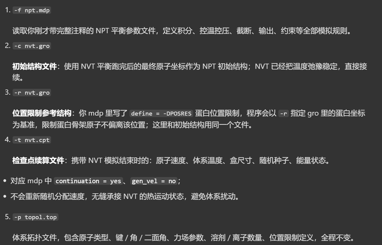
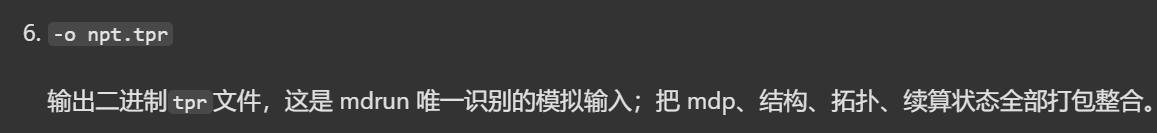
第一步输出日志如下
python
Executable:   /home/csn/program/miniconda3/envs/tf-dna-md/bin.AVX2_256/gmx
Data prefix:  /home/csn/program/miniconda3/envs/tf-dna-md
Working dir:  /mnt/sdb/zht/project/tf-dna-md/files/structure
Command line:
  gmx grompp -f npt.mdp -c nvt.gro -r nvt.gro -t nvt.cpt -p topol.top -o npt.tpr

Ignoring obsolete mdp entry 'title'
Ignoring obsolete mdp entry 'ns_type'
Setting the LD random seed to 2079319487

# 随机种子、非键作用、1-4 相互作用构建
Generated 169542 of the 169653 non-bonded parameter combinations
Generating 1-4 interactions: fudge = 1

Generated 118878 of the 169653 1-4 parameter combinations

Excluding 3 bonded neighbours molecule type 'Protein_chain_A'

# 氢键约束生效(对应 mdp constraints = h-bonds)
turning H bonds into constraints...

Excluding 2 bonded neighbours molecule type 'SOL'

turning H bonds into constraints...

Excluding 3 bonded neighbours molecule type 'CL'

turning H bonds into constraints...

# ⚠️ 速度来源:读取 NVT 末态速度(对应 -t nvt.cpt、gen_vel=no)
Taking velocities from 'nvt.gro'
Analysing residue names:
# 体系构成:129 个溶菌酶残基 + 12589 水分子 + 8 个氯离子;全体系统一温控,自由度正常
There are:   129    Protein residues
There are: 12589      Water residues
There are:     8        Ion residues
Analysing Protein...
Number of degrees of freedom in T-Coupling group System is 80476.00

The largest distance between excluded atoms is 0.452 nm between atom 1156 and 1405

# Verlet 邻域列表缓冲计算
Determining Verlet buffer for a tolerance of 0.005 kJ/mol/ps at 298 K

Calculated rlist for 1x1 atom pair-list as 1.234 nm, buffer size 0.034 nm

Set rlist, assuming 4x4 atom pair-list, to 1.200 nm, buffer size 0.000 nm

Note that mdrun will redetermine rlist based on the actual pair-list setup

  rest:          3.687  3.719  3.704
  rest:          3.687  3.719  3.704

NOTE 1 [file npt.mdp]:
  Removing center of mass motion in the presence of position restraints
  might cause artifacts. When you are using position restraints to
  equilibrate a macro-molecule, the artifacts are usually negligible.

# 成功读取 NVT 模拟终点(100 ps)的坐标、速度、盒子尺寸
Reading Coordinates, Velocities and Box size from old trajectory

Will read whole trajectory
Last frame         -1 time  100.000

Using frame at t = 100 ps

# NPT 模拟内部计时从 0 ps 重新开始,物理上无缝接续 NVT 热运动状态
Starting time for run is 0 ps
# PME 傅里叶网格(长程静电)
Calculating fourier grid dimensions for X Y Z
Using a fourier grid of 48x48x48, spacing 0.154 0.154 0.154

Estimate for the relative computational load of the PME mesh part: 0.15

This run will generate roughly 461 Mb of data

There was 1 NOTE
然后我们开始模拟,因为这一步耗时比较长,所以我放在tmux中运行

实测跑了将近1个小时,
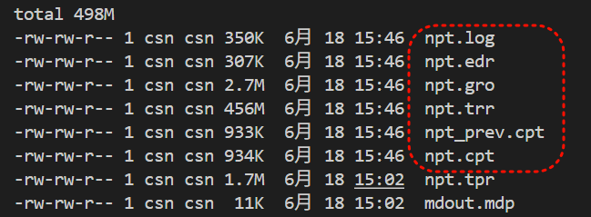
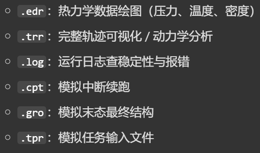
日志如下
python
Executable:   /home/csn/program/miniconda3/envs/tf-dna-md/bin.AVX2_256/gmx
Data prefix:  /home/csn/program/miniconda3/envs/tf-dna-md
Working dir:  /mnt/sdb/zht/project/tf-dna-md/files/structure
Command line:
  gmx mdrun -deffnm npt

Compiled SIMD is AVX2_256, but AVX_512 might be faster (see log).
The current CPU can measure timings more accurately than the code in
gmx mdrun was configured to use. This might affect your simulation
speed as accurate timings are needed for load-balancing.
Please consider rebuilding gmx mdrun with the GMX_USE_RDTSCP=ON CMake option.
Reading file npt.tpr, VERSION 2025.4-conda_forge (single precision)
Changing nstlist from 10 to 80, rlist from 1.2 to 1.322


Using 32 MPI threads
Using 1 OpenMP thread per tMPI thread

starting mdrun 'LYSOZYME in water'
250000 steps,    500.0 ps.

Writing final coordinates.


Dynamic load balancing report:
 DLB was turned on during the run due to measured imbalance.
 Average load imbalance: 24.3%.
 The balanceable part of the MD step is 63%, load imbalance is computed from this.
 Part of the total run time spent waiting due to load imbalance: 15.3%.
 Steps where the load balancing was limited by -rdd, -rcon and/or -dds: X 0 % Y 0 % Z 0 %
 Average PME mesh/force load: 0.650
 Part of the total run time spent waiting due to PP/PME imbalance: 7.1 %

NOTE: 15.3 % of the available CPU time was lost due to load imbalance
      in the domain decomposition.
      You can consider manually changing the decomposition (option -dd);
      e.g. by using fewer domains along the box dimension in which there is
      considerable inhomogeneity in the simulated system.
NOTE: 7.1 % performance was lost because the PME ranks
      had less work to do than the PP ranks.
      You might want to decrease the number of PME ranks
      or decrease the cut-off and the grid spacing.


               Core t (s)   Wall t (s)        (%)
       Time:    59975.465     1874.235     3200.0
                         31:14
                 (ns/day)    (hour/ns)
Performance:       23.049        1.041

GROMACS reminds you: "C has the power of assembly language and the convenience of... assembly language." (Dennis Ritchie)
然后同样的,我们再次进行能量分析
因为这回我们是要看压力变化情况,
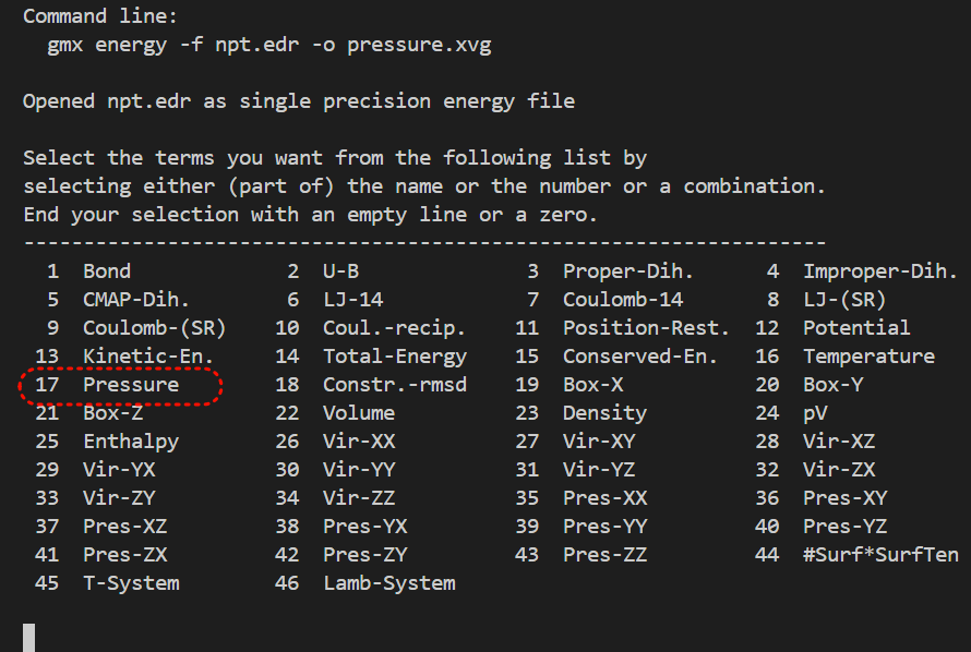
输出日志如下,一并中文注释
python
Executable:   /home/csn/program/miniconda3/envs/tf-dna-md/bin.AVX2_256/gmx
Data prefix:  /home/csn/program/miniconda3/envs/tf-dna-md
Working dir:  /mnt/sdb/zht/project/tf-dna-md/files/structure
Command line:
  gmx energy -f npt.edr -o pressure.xvg

Opened npt.edr as single precision energy file

Select the terms you want from the following list by
selecting either (part of) the name or the number or a combination.
End your selection with an empty line or a zero.
-------------------------------------------------------------------
  1  Bond             2  U-B              3  Proper-Dih.      4  Improper-Dih.
  5  CMAP-Dih.        6  LJ-14            7  Coulomb-14       8  LJ-(SR)
  9  Coulomb-(SR)    10  Coul.-recip.    11  Position-Rest.  12  Potential
 13  Kinetic-En.     14  Total-Energy    15  Conserved-En.   16  Temperature
 17  Pressure        18  Constr.-rmsd    19  Box-X           20  Box-Y
 21  Box-Z           22  Volume          23  Density         24  pV
 25  Enthalpy        26  Vir-XX          27  Vir-XY          28  Vir-XZ
 29  Vir-YX          30  Vir-YY          31  Vir-YZ          32  Vir-ZX
 33  Vir-ZY          34  Vir-ZZ          35  Pres-XX         36  Pres-XY
 37  Pres-XZ         38  Pres-YX         39  Pres-YY         40  Pres-YZ
 41  Pres-ZX         42  Pres-ZY         43  Pres-ZZ         44  #Surf*SurfTen
 45  T-System        46  Lamb-System

17 0
Last energy frame read 500 time  500.000

Statistics over 250001 steps [ 0.0000 through 500.0000 ps ], 1 data sets
All statistics are over 2501 points

# Average 平均值:-16.9879 bar
# 目标平衡压力是 1 bar,平均压力远偏离常压,说明500 ps NPT 没有平衡到位。压力平均值为负值代表盒子整体偏小,分子间排斥力不足,体系有膨胀趋势。
# Err.Est. 误差估计:12 bar
# 压力波动的统计误差很大,曲线震荡幅度极高
# RMSD 均方根偏差:144.336 bar
# 全程压力存在明显单向漂移,500 ps 结束时压力和初始阶段差距很大,体系密度未收敛稳定
#
    Energy                      Average   Err.Est.       RMSD  Tot-Drift
-------------------------------------------------------------------------------
Pressure                   -16.9879         12    144.336    42.5112  (bar)

GROMACS reminds you: "Move Over Hogey Bear" (Urban Dance Squad)
只生成了1个xvg文件,
我们这里选用GMXvg工具作为测试示例,
https://github.com/TheBiomics/GMXvg
注意python版本限制,不要太高,不然会有版本语法报错
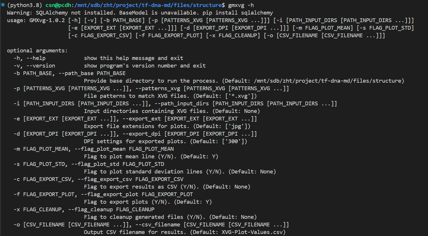
python
# 安装
pip install gmxvg
# 单个xvg目录下测试,或批量
gmxvg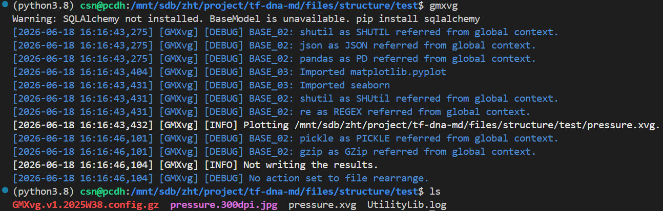
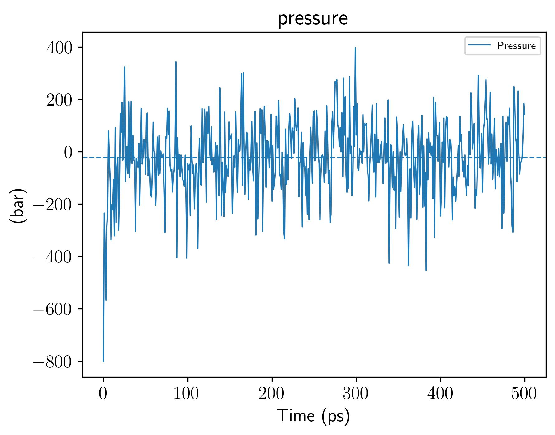
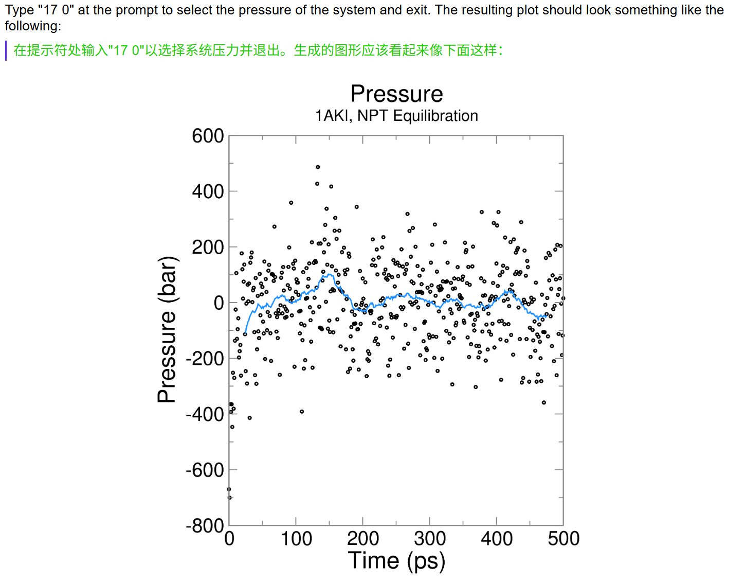
基本上差不多,
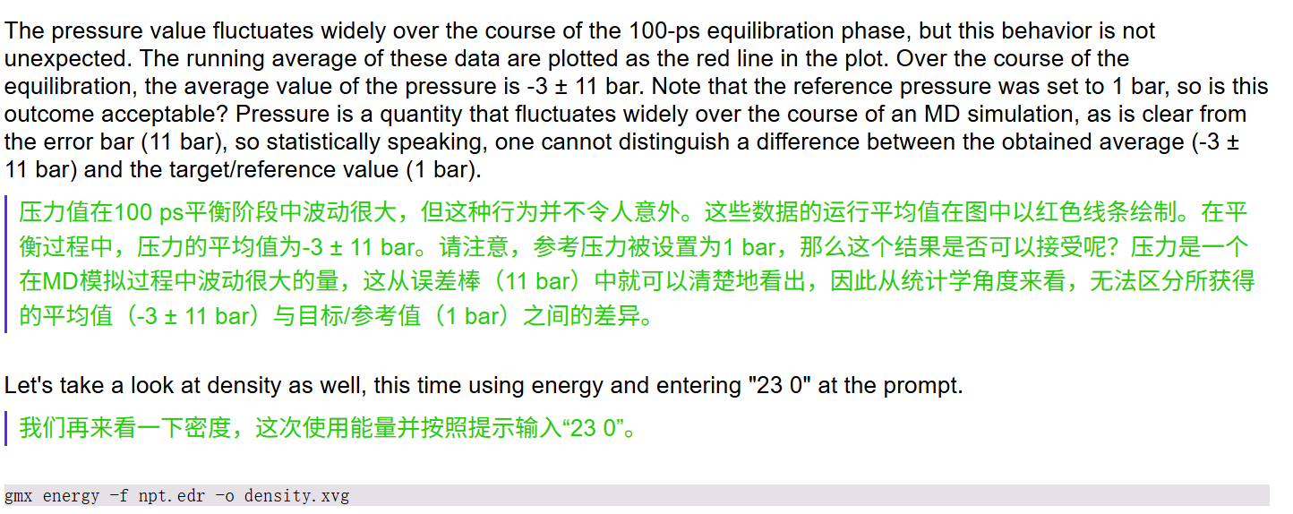
我们命令如下
python
gmx energy -f npt.edr -o density.xvg输入日志如下
python
Executable:   /home/csn/program/miniconda3/envs/tf-dna-md/bin.AVX2_256/gmx
Data prefix:  /home/csn/program/miniconda3/envs/tf-dna-md
Working dir:  /mnt/sdb/zht/project/tf-dna-md/files/structure
Command line:
  gmx energy -f npt.edr -o density.xvg

Opened npt.edr as single precision energy file

Select the terms you want from the following list by
selecting either (part of) the name or the number or a combination.
End your selection with an empty line or a zero.
-------------------------------------------------------------------
  1  Bond             2  U-B              3  Proper-Dih.      4  Improper-Dih.
  5  CMAP-Dih.        6  LJ-14            7  Coulomb-14       8  LJ-(SR)
  9  Coulomb-(SR)    10  Coul.-recip.    11  Position-Rest.  12  Potential
 13  Kinetic-En.     14  Total-Energy    15  Conserved-En.   16  Temperature
 17  Pressure        18  Constr.-rmsd    19  Box-X           20  Box-Y
 21  Box-Z           22  Volume          23  Density         24  pV
 25  Enthalpy        26  Vir-XX          27  Vir-XY          28  Vir-XZ
 29  Vir-YX          30  Vir-YY          31  Vir-YZ          32  Vir-ZX
 33  Vir-ZY          34  Vir-ZZ          35  Pres-XX         36  Pres-XY
 37  Pres-XZ         38  Pres-YX         39  Pres-YY         40  Pres-YZ
 41  Pres-ZX         42  Pres-ZY         43  Pres-ZZ         44  #Surf*SurfTen
 45  T-System        46  Lamb-System

23 0
Last energy frame read 500 time  500.000

Statistics over 250001 steps [ 0.0000 through 500.0000 ps ], 1 data sets
All statistics are over 2501 points

Energy                      Average   Err.Est.       RMSD  Tot-Drift
-------------------------------------------------------------------------------
Density                     1024.58       0.75    4.11748    2.75266  (kg/m^3)

GROMACS reminds you: "The only place success comes before work is in the dictionary" (Vince Lombardi)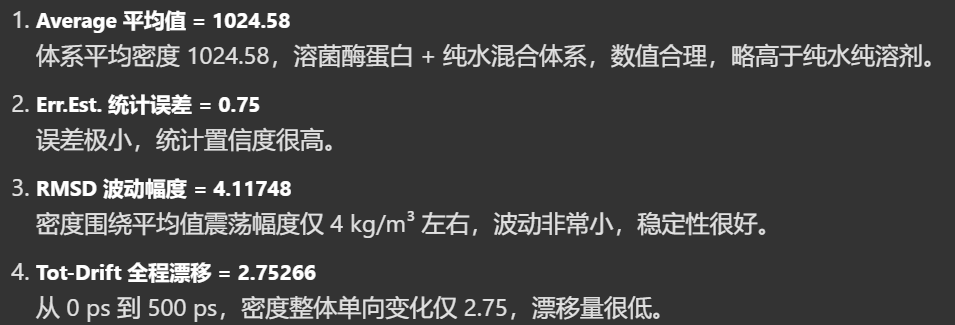

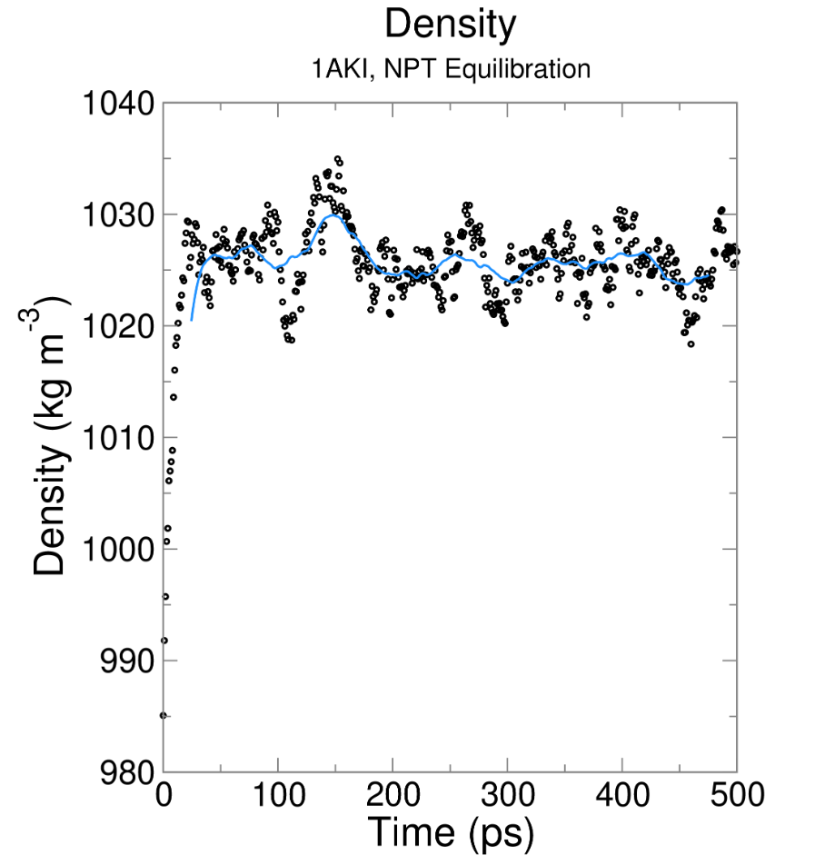
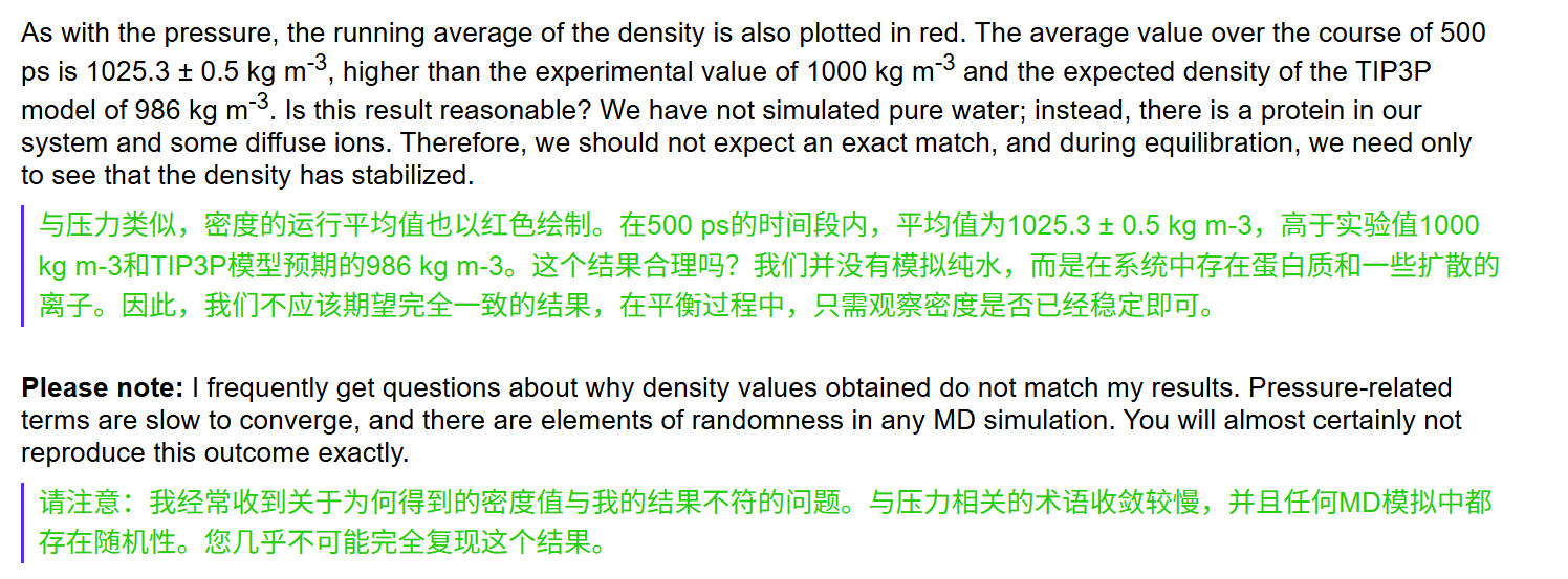
这里可视化xvg文件,我开发了一个小工具,因为觉得和前面那样脚本处理太麻烦了,暂时有没有找到什么趁手的仓库工具。
参考仓库:https://github.com/MaybeBio/gmxplot
初版比较粗糙,目前安装在r-jupyter环境中
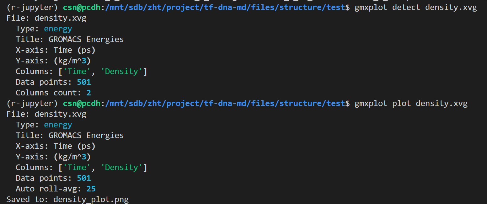
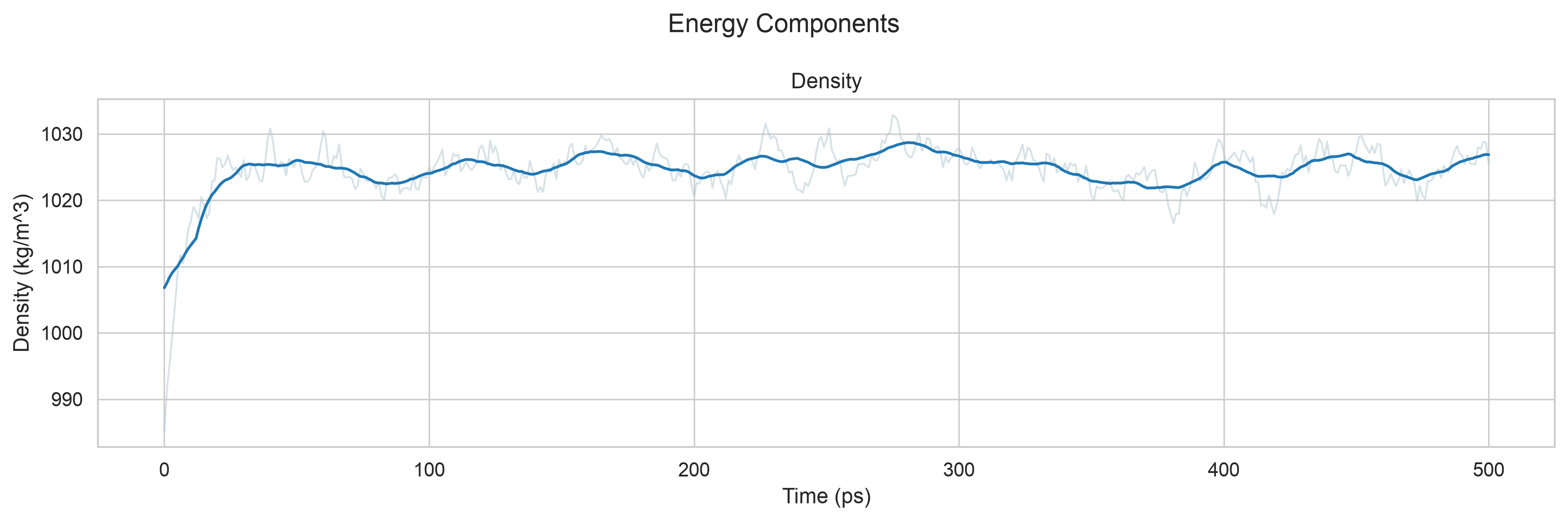
还是那句话,比较粗糙,但是能看,目前演示阶段还没有深入优化,只是简单查看一下数据
7,Production MD 正式MD模拟
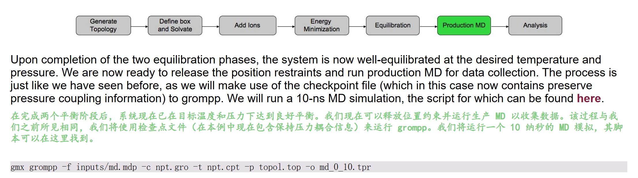
同样的,我们运行gmx grompp命令,这里同样使用教程提供的mdp配置文件,
参考:http://www.mdtutorials.com/gmx/lysozyme/Files/md.mdp
python
title                   = OPLS Lysozyme MD run
; Run parameters
integrator              = md        ; leap-frog integrator
nsteps                  = 5000000   ; 2 * 2500000 = 10000 ps (10 ns)
dt                      = 0.002     ; 2 fs
; Output control
nstxout                 = 0         ; suppress bulky .trr file by specifying
nstvout                 = 0         ; 0 for output frequency of nstxout,
nstfout                 = 0         ; nstvout, and nstfout
nstenergy               = 5000      ; save energies every 10.0 ps
nstlog                  = 5000      ; update log file every 10.0 ps
nstxout-compressed      = 5000      ; save compressed coordinates every 10.0 ps
compressed-x-grps       = System    ; save the whole system
; Bond parameters
continuation            = yes       ; Restarting after NPT
constraint_algorithm    = lincs     ; holonomic constraints
constraints             = h-bonds   ; bonds involving H are constrained
lincs_iter              = 1         ; accuracy of LINCS
lincs_order             = 4         ; also related to accuracy
; Nonbonded settings
cutoff-scheme           = Verlet    ; Buffered neighbor searching
ns_type                 = grid      ; search neighboring grid cells
nstlist                 = 10        ; 20 fs, largely irrelevant with Verlet scheme
; vdW
rvdw                    = 1.2       ; short-range van der Waals cutoff (in nm)
rvdw-switch             = 1.0
vdw-modifier            = force-switch
DispCorr                = No
; Electrostatics
rcoulomb                = 1.2       ; short-range electrostatic cutoff (in nm)
coulombtype             = PME       ; Particle Mesh Ewald for long-range electrostatics
pme_order               = 4         ; cubic interpolation
fourierspacing          = 0.16      ; grid spacing for FFT
; Temperature coupling is on
tcoupl                  = V-rescale             ; modified Berendsen thermostat
tc-grps                 = System
tau_t                   = 1.0
ref_t                   = 298
; Pressure coupling is on
pcoupl                  = C-rescale
pcoupltype              = isotropic             ; uniform scaling of box vectors
tau_p                   = 5.0                   ; time constant, in ps
ref_p                   = 1.0                   ; reference pressure, in bar
compressibility         = 4.5e-5                ; isothermal compressibility of water, bar^-1
; Periodic boundary conditions
pbc                     = xyz       ; 3-D PBC
; Velocity generation
gen_vel                 = no        ; Velocity generation is off
python
# ====================== 前置说明 ======================
# Upon completion of the two equilibration phases, the system is now well-equilibrated at the desired temperature and pressure.
# 在完成NVT、NPT两步平衡阶段后,体系已在目标温度、压力下充分平衡
# We are now ready to release the position restraints and run production MD for data collection.
# 本生产模拟文件已移除蛋白位置约束,用于采集可统计动力学轨迹数据
# The process is just like we have seen before, as we will make use of the checkpoint file (which in this case now contains preserve pressure coupling information) to grompp.
# 预处理时需传入NPT平衡的.cpt检查点文件,继承温度、压力耦合、原子速度等完整热力学信息
# We will run a 10-ns MD simulation, the script for which can be found here.
# 本参数总模拟时长10 ns,配套预处理命令:
# gmx grompp -f inputs/md.mdp -c npt.gro -t npt.cpt -p topol.top -o md_0_10.tpr
# ======================================================

title                   = OPLS Lysozyme MD run  ; 模拟任务名称:OPLS力场溶菌酶生产动力学模拟

;==================== 模拟核心运行参数 ====================
integrator              = md        ; 积分器:leap-frog蛙跳算法,标准分子动力学积分方案
nsteps                  = 5000000   ; 总模拟步数500万步,dt=2fs,总时长5e6*0.002=10000ps=10ns
dt                      = 0.002     ; 积分步长2飞秒,约束氢键后安全步长,兼顾效率与稳定性

;==================== 轨迹&能量输出控制 ====================
nstxout                 = 0         ; 不输出无压缩完整.trr轨迹文件(体积大,仅保留压缩轨迹)
nstvout                 = 0         ; 不输出速度轨迹文件,减少磁盘占用
nstfout                 = 0         ; 不输出受力轨迹文件,生产模拟无需记录受力
nstenergy               = 5000      ; 每5000步(10ps)输出能量数据(势能、动能、温压、范德华/静电能等)
nstlog                  = 5000      ; 每5000步更新日志log文件,实时监控模拟运行状态
nstxout-compressed      = 5000      ; 每5000步(10ps)输出压缩.xtc坐标轨迹,用于后续构象分析
compressed-x-grps       = System    ; 压缩轨迹保存整个体系所有原子,方便完整体系分析

;==================== 键约束 & 续跑设置 ====================
continuation            = yes       ; 开启续跑模式,从NPT平衡末态继续模拟,复用检查点速度/温压信息
constraint_algorithm    = lincs     ; 约束求解算法LINCS,适合蛋白大分子体系,精度高
constraints             = h-bonds   ; 约束所有含氢原子化学键(C-H/O-H/N-H),允许2fs大步长
lincs_iter              = 1         ; LINCS约束迭代次数,常规体系1次足够
lincs_order             = 4         ; LINCS高阶校正阶数,4阶消除键拉伸伪影,保证约束精度

;==================== 非键相互作用(范德华vdW) ====================
cutoff-scheme           = Verlet    ; 邻居列表方案Verlet缓冲列表,现代GROMACS推荐,计算稳定高效
ns_type                 = grid      ; 网格法搜索邻近原子,加速邻居列表构建
nstlist                 = 10        ; 每10步更新一次邻居列表,Verlet方案下该参数影响很小
rvdw                    = 1.2       ; 范德华短程截断半径1.2 nm
rvdw-switch             = 1.0       ; 范德华力切换起始距离1.0 nm,1.0~1.2nm作用力平滑衰减至0
vdw-modifier            = force-switch ; 力切换模式,仅作用力平滑衰减,能量连续无突变
DispCorr                = No        ; 关闭长程色散校正,OPLS蛋白水溶液模拟常用设置

;==================== 静电相互作用 ====================
rcoulomb                = 1.2       ; 静电短程截断半径与vdW统一为1.2 nm
coulombtype             = PME       ; 粒子网格埃瓦尔德PME,精准计算长程静电相互作用,水溶液体系标准
pme_order               = 4         ; PME插值阶数4次立方插值,平衡精度与计算开销
fourierspacing          = 0.16      ; PME傅里叶网格间距0.16nm,网格越密静电精度越高

;==================== 温度耦合控温 ====================
tcoupl                  = V-rescale             ; 温控算法V-rescale(修正Berendsen),速度重缩放,温度波动小
tc-grps                 = System  ; 整个体系作为单一温控组(蛋白+水+离子统一控温298K)
tau_t                   = 1.0                   ; 温控时间常数1ps,耦合强度适中,快速稳定温度
ref_t                   = 298                   ; 目标参考温度298 K(25℃室温)

;==================== 压力耦合控压 ====================
pcoupl                  = C-rescale  ; 压控算法C-rescale,适配续跑NPT平衡体系,盒子缩放稳定
pcoupltype              = isotropic             ; 各向同性压耦,x/y/z三个方向盒子同步缩放
tau_p                   = 5.0                   ; 压控时间常数5ps,压力弛豫速度平缓,避免震荡
ref_p                   = 1.0                   ; 目标参考压力1 bar(标准大气压)
compressibility         = 4.5e-5                ; 水的等温压缩系数,单位bar⁻¹,用于压力盒子缩放计算

;==================== 周期性边界条件 & 速度生成 ====================
pbc                     = xyz       ; x/y/z三维周期性边界,模拟无限水溶液环境,消除表面效应
gen_vel                 = no        ; 不重新生成原子速度,复用npt.cpt检查点内已平衡的速度场
然后我们的运行命令如下:
python
gmx grompp -f md.mdp -c npt.gro -t npt.cpt -p topol.top -o md_0_10.tpr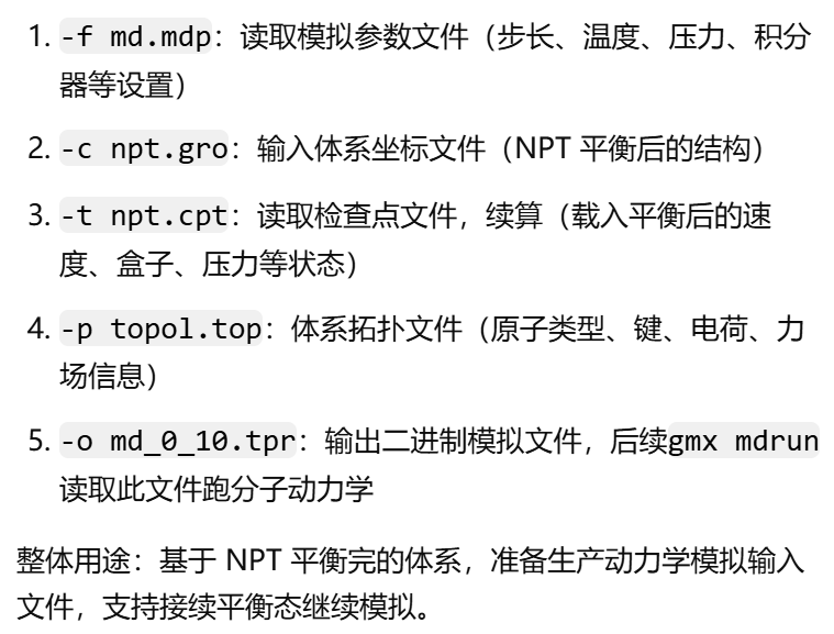
然后执行日志如下:
- 两步平衡(NVT 恒温恒容平衡 + NPT 恒温恒压平衡)全部跑完后,体系温度、压力、盒子密度、势能、分子运动全部稳定在设定值(298 K、1 bar),无大幅漂移震荡,达到热力学平衡状态。
- 平衡阶段为防止蛋白结构崩坏,一般会给蛋白主链 / 重原子加位置约束 posres;生产模拟要观测蛋白真实构象波动,必须解除位置约束。当前 mdp 与拓扑文件已关闭约束,可自由采集轨迹做后续分析(RMSD、RMSF、氢键、结合作用、构象聚类等)
python
#
Executable:   /home/csn/program/miniconda3/envs/tf-dna-md/bin.AVX2_256/gmx
Data prefix:  /home/csn/program/miniconda3/envs/tf-dna-md
Working dir:  /mnt/sdb/zht/project/tf-dna-md/files/structure
Command line:
  gmx grompp -f md.mdp -c npt.gro -t npt.cpt -p topol.top -o md_0_10.tpr

Ignoring obsolete mdp entry 'title'
Ignoring obsolete mdp entry 'ns_type'

# 随机种子与非键、1-4 作用参数构建
Setting the LD random seed to -675286025

Generated 169542 of the 169653 non-bonded parameter combinations
Generating 1-4 interactions: fudge = 1

Generated 118878 of the 169653 1-4 parameter combinations

# 分子键约束处理(仅约束氢键,无蛋白位置约束)
# 分别对蛋白、水分子、氯离子体系启用 constraints = h-bonds,约束所有含氢化学键
Excluding 3 bonded neighbours molecule type 'Protein_chain_A'

turning H bonds into constraints...

Excluding 2 bonded neighbours molecule type 'SOL'

turning H bonds into constraints...

Excluding 3 bonded neighbours molecule type 'CL'

turning H bonds into constraints...

# 读取平衡末态速度、结构、统计体系组分
# 从 NPT 平衡结果继承速度,不重新生成(gen_vel=no)
Taking velocities from 'npt.gro'
Analysing residue names:
# 体系组分统计:129 个溶菌酶残基、12589 个水分子、8 个氯离子;
There are:   129    Protein residues
There are: 12589      Water residues
There are:     8        Ion residues
Analysing Protein...
# 温控自由度:整个体系统一温控组 System,总自由度 80476,用于 V-rescale 温控计算温度
Number of degrees of freedom in T-Coupling group System is 80476.00

# 邻居列表 Verlet 缓冲计算
# 根据 298K 温度、力误差阈值自动计算 Verlet 邻居列表缓冲;运行 mdrun 时会动态调整邻居列表半径,保证截断 1.2 nm 内作用力计算精度
The largest distance between excluded atoms is 0.440 nm between atom 1156 and 1405

Determining Verlet buffer for a tolerance of 0.005 kJ/mol/ps at 298 K

Calculated rlist for 1x1 atom pair-list as 1.234 nm, buffer size 0.034 nm

Set rlist, assuming 4x4 atom pair-list, to 1.200 nm, buffer size 0.000 nm

Note that mdrun will redetermine rlist based on the actual pair-list setup

# 读取 NPT 平衡末态时间,设定生产模拟起点
# NPT 平衡总时长 500 ps,取最后一帧作为生产模拟初始态
# 生产模拟内部计时从 0 ps 开始,累计运行 10 ns;物理时间等价接续在 500 ps 平衡之后
Reading Coordinates, Velocities and Box size from old trajectory

Will read whole trajectory
Last frame         -1 time  500.000

Using frame at t = 500 ps

Starting time for run is 0 ps
# PME 静电网格计算
# PME 傅里叶网格 48×48×48,实际网格间距 0.152 nm,接近 mdp 设定 0.16 nm
# PME 网格计算仅占总算力 15%,计算压力小,模拟速度快
Calculating fourier grid dimensions for X Y Z
Using a fourier grid of 48x48x48, spacing 0.152 0.152 0.152

Estimate for the relative computational load of the PME mesh part: 0.15
# 10 ns 模拟按每 10 ps 输出一帧 xtc 轨迹 + 能量文件,总输出文件约 197MB
This run will generate roughly 197 Mb of data

GROMACS reminds you: "Science is a way of thinking much more than it is a body of knowledge." (Carl Sagan)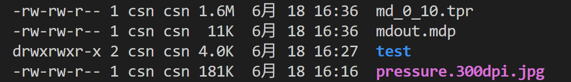
然后我们再开始模拟
python
gmx mdrun -deffnm md_0_10运行日志如下:
python
Executable:   /home/csn/program/miniconda3/envs/tf-dna-md/bin.AVX2_256/gmx
Data prefix:  /home/csn/program/miniconda3/envs/tf-dna-md
Working dir:  /mnt/sdb/zht/project/tf-dna-md/files/structure
Command line:
  gmx mdrun -deffnm md_0_10

Compiled SIMD is AVX2_256, but AVX_512 might be faster (see log).
The current CPU can measure timings more accurately than the code in
gmx mdrun was configured to use. This might affect your simulation
speed as accurate timings are needed for load-balancing.
Please consider rebuilding gmx mdrun with the GMX_USE_RDTSCP=ON CMake option.
Reading file md_0_10.tpr, VERSION 2025.4-conda_forge (single precision)
Changing nstlist from 10 to 80, rlist from 1.2 to 1.324


Using 32 MPI threads
Using 1 OpenMP thread per tMPI thread

starting mdrun 'LYSOZYME in water'
5000000 steps,  10000.0 ps.

Writing final coordinates.


Dynamic load balancing report:
 DLB got disabled because it was unsuitable to use.
 Average load imbalance: 18.2%.
 The balanceable part of the MD step is 70%, load imbalance is computed from this.
 Part of the total run time spent waiting due to load imbalance: 12.8%.
 Average PME mesh/force load: 0.546
 Part of the total run time spent waiting due to PP/PME imbalance: 9.6 %

NOTE: 12.8 % of the available CPU time was lost due to load imbalance
      in the domain decomposition.
      You can consider manually changing the decomposition (option -dd);
      e.g. by using fewer domains along the box dimension in which there is
      considerable inhomogeneity in the simulated system.
NOTE: 9.6 % performance was lost because the PME ranks
      had less work to do than the PP ranks.
      You might want to decrease the number of PME ranks
      or decrease the cut-off and the grid spacing.


               Core t (s)   Wall t (s)        (%)
       Time:   677303.396    21165.734     3200.0
                         5h52:45
                 (ns/day)    (hour/ns)
Performance:       40.821        0.588

GROMACS reminds you: "We haven't the money, so we've got to think." (Ernest Rutherford)
注释一并整合
python
# ===================== mdrun 完整运行日志 + 逐行注释 =====================
Executable:   /home/csn/program/miniconda3/envs/tf-dna-md/bin.AVX2_256/gmx  ; 程序路径:conda环境AVX2_256向量化编译版GROMACS
Data prefix:  /home/csn/program/miniconda3/envs/tf-dna-md                  ; GMX库、力场文件根目录
Working dir:  /mnt/sdb/zht/project/tf-dna-md/files/structure              ; 模拟工作目录,存放tpr、轨迹、能量文件
Command line:   gmx mdrun -deffnm md_0_10                                 ; 运行指令,-deffnm统一文件前缀md_0_10,自动读写md_0_10.tpr、xtc、edr、log、cpt等

Compiled SIMD is AVX2_256, but AVX_512 might be faster (see log).
; 当前CPU仅支持AVX2 256位向量加速;若CPU支持AVX512重新编译可进一步提升单核速度
The current CPU can measure timings more accurately than the code in gmx mdrun was configured to use.
This might affect your simulation speed as accurate timings are needed for load-balancing.
Please consider rebuilding gmx mdrun with the GMX_USE_RDTSCP=ON CMake option.
; 编译时未开启高精度CPU时钟计时RDTSCP,动态负载均衡(DLB)计时不准;重新编译开启GMX_USE_RDTSCP可改善负载均衡判定

Reading file md_0_10.tpr, VERSION 2025.4-conda_forge (single precision)
; 读取预处理生成的二进制运行文件tpr,GMX版本2025.4 conda编译,单精度浮点计算(生物模拟标准)

Changing nstlist from 10 to 80, rlist from 1.2 to 1.324
; mdrun自动优化邻居列表参数:
; mdp中nstlist=10,运行时自动改为80步更新一次邻居列表;
; Verlet缓冲列表半径rlist由截断1.2nm拓宽至1.324nm,减少频繁重建邻居列表开销,平衡精度与速度

Using 32 MPI threads
Using 1 OpenMP thread per tMPI thread
; 并行架构:32个MPI域分解进程,每个MPI进程绑定1个OpenMP线程,总CPU核心占用32核

starting mdrun 'LYSOZYME in water'
5000000 steps,  10000.0 ps.
; 开始运行溶菌酶水溶液生产模拟,总步数500万步,总模拟时长10000 ps = 10 ns,与mdp参数完全对应
Writing final coordinates.
; 模拟全部步数跑完,正在输出最后一帧坐标、检查点文件

Dynamic load balancing report:  ; 动态负载均衡DLB报告
DLB got disabled because it was unsuitable to use.
; 程序自动关闭动态负载均衡:体系分布不均(蛋白集中在盒子局部,水充斥其余区域),DLB收益低于通讯开销
Average load imbalance: 18.2%.
; 平均域负载不均衡度18.2%,各CPU核心计算任务量差距较大
The balanceable part of the MD step is 70%, load imbalance is computed from this.
; MD迭代中70%计算量可被负载均衡优化,不均衡度基于该部分统计
Part of the total run time spent waiting due to load imbalance: 12.8%.
; 因CPU任务分配不均产生的空闲等待时间,占总运行时长12.8%,性能损耗明显

Average PME mesh/force load: 0.546
Part of the total run time spent waiting due to PP/PME imbalance: 9.6 %
; PP=短程力计算(范德华、键合作用),PME=长程静电网格计算
; PME进程平均负载仅为PP进程的0.546倍,PME算力闲置;PP/PME任务不均衡造成9.6%额外等待损耗

NOTE: 12.8 % of the available CPU time was lost due to load imbalance in the domain decomposition.
You can consider manually changing the decomposition (option -dd);
e.g. by using fewer domains along the box dimension in which there is considerable inhomogeneity in the simulated system.
; 提示1:域分解不均衡损耗12.8%算力;可手动通过-dd指定三维域划分数量,在蛋白分布集中的维度减少MPI划分块数,缓解负载倾斜

NOTE: 9.6 % performance was lost because the PME ranks had less work to do than the PP ranks.
You might want to decrease the number of PME ranks or decrease the cut-off and the grid spacing.
; 提示2:PME进程算力闲置损耗9.6%;优化方案:减少PME并行进程数、适当降低截断半径、缩小PME网格间距平衡PP/PME计算量

                  Core t (s)   Wall t (s)        (%)
        Time:   677303.396    21165.734     3200.0
                          5h52:45
; Core t:所有CPU核心累计总计算时长 677303 s
; Wall t:实际墙上时钟运行总时长 21165.734 s ≈ 5小时52分45秒
; (%)=3200:总核心算力倍数(32核并行,理论加速32倍,实际因通讯、负载均衡损耗未达理论峰值)

                  (ns/day)    (hour/ns)
Performance:       40.821        0.588
; 模拟性能指标:
; 40.821 ns/day:每日可完成40.821纳秒模拟
; 0.588 hour/ns:每1纳秒模拟需要0.588小时CPU墙上时间
; 对比前文GPU预期196 ns/day,纯CPU并行速度仅为GPU的1/5左右
可以看到,模拟这个10ns过程大概花费了6个小时(还是32核并行)
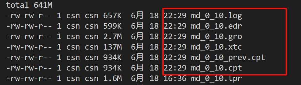
我们可以知道:
- 键相互作用:在cpu上计算
- 非键相互作用/PME:在gpu上计算
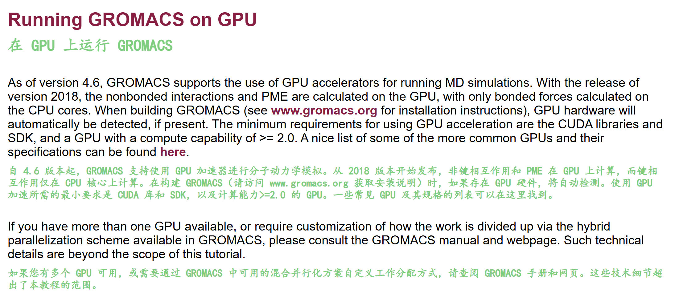
⚠️ 这里比较闹乌龙的一点是,我跑到这里才发现我之前的mdrun模拟中PME和非键相互作用都没有用上gpu,然后回头去才发现我在conda yml配置文件中并没有显式选择1个cuda版的gromacs。
所以,这里我又回去修改了一下我的环境配置(主要是gromacs的配置,以及其他冲突环境),
参考我之前的博客Gromacs笔记 - 01 安装,
之前是在tf-dna-md跑,但是没有gpu支持,现在改成gmx-mpi为tf-dna-md环境,我们后续在gromacs环境中运行教程
总之,在修改了配置之后,我们再运行,可以看到确实是支持了gpu
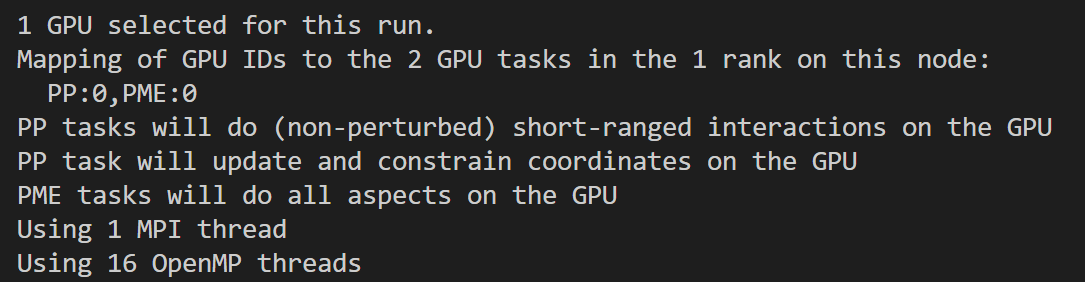
python
# 配置都可以看到
nvitop
nvidia-smi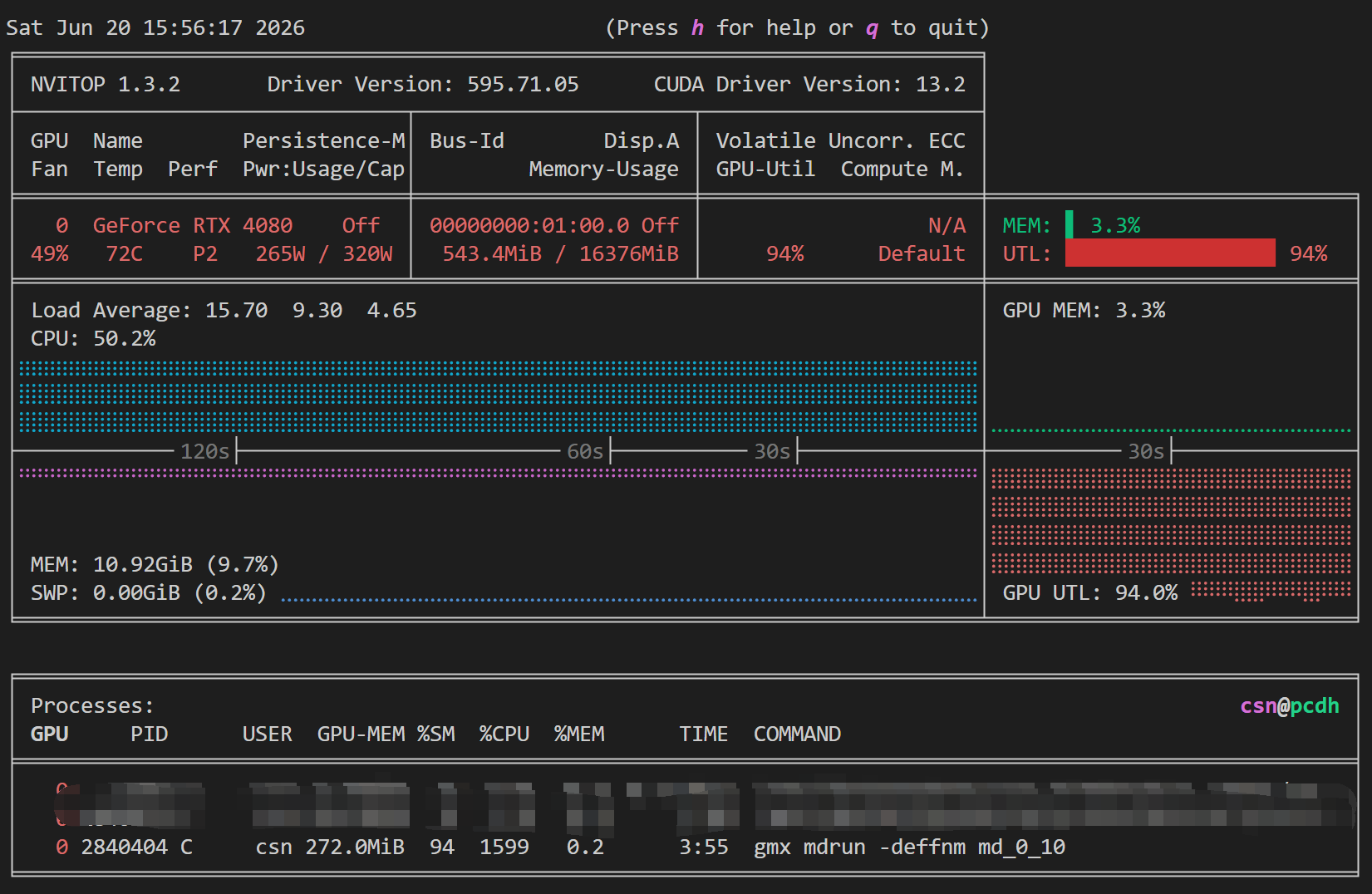
现在重新运行之后的日志如下
python
Executable:   /home/csn/program/miniconda3/envs/gromacs/bin.AVX2_256/gmx
Data prefix:  /home/csn/program/miniconda3/envs/gromacs
Working dir:  /mnt/sdb/zht/project/tf-dna-md/files/structure/test
Command line:
  gmx mdrun -deffnm md_0_10


Back Off! I just backed up md_0_10.log to ./#md_0_10.log.1#
Compiled SIMD is AVX2_256, but AVX_512 might be faster (see log).
The current CPU can measure timings more accurately than the code in
gmx mdrun was configured to use. This might affect your simulation
speed as accurate timings are needed for load-balancing.
Please consider rebuilding gmx mdrun with the GMX_USE_RDTSCP=ON CMake option.
Reading file md_0_10.tpr, VERSION 2025.4-conda_forge (single precision)
Changing nstlist from 10 to 100, rlist from 1.2 to 1.352


1 GPU selected for this run.
Mapping of GPU IDs to the 2 GPU tasks in the 1 rank on this node:
  PP:0,PME:0
PP tasks will do (non-perturbed) short-ranged interactions on the GPU
PP task will update and constrain coordinates on the GPU
PME tasks will do all aspects on the GPU
Using 1 MPI thread
Using 16 OpenMP threads

starting mdrun 'LYSOZYME in water'
5000000 steps,  10000.0 ps.

Writing final coordinates.

               Core t (s)   Wall t (s)        (%)
       Time:    22476.793     1404.801     1600.0
                 (ns/day)    (hour/ns)
Performance:      615.034        0.039

GROMACS reminds you: "You Could Make More Money As a Butcher" (F. Zappa)
一并中文注释如下
python
# ====================== 日志分段逐行解读 + GPU vs CPU 核心对比 ======================
# 1. 程序编译与SIMD指令集信息
Executable:   /home/csn/program/miniconda3/envs/gromacs/bin.AVX2_256/gmx
Data prefix:  /home/csn/program/miniconda3/envs/gromacs
# 编译分支为AVX2_256单精度GPU版,提示CPU支持AVX512但当前二进制未编译;
# 【CPU版对比】纯CPU编译若开启AVX512,单核CPU计算理论浮点更高,但无GPU加速核心,总算力上限由CPU核心数锁定;
# 同时日志提示编译开启GMX_USE_RDTSCP可提升计时精度,CPU负载均衡、GPU负载均衡均受益,GPU多任务调度对计时精度更敏感。

# 2. 运行路径与备份机制
Working dir:  /mnt/sdb/zht/project/tf-dna-md/files/structure/test
Command line: gmx mdrun -deffnm md_0_10
Back Off! I just backed up md_0_10.log to ./#md_0_10.log.1#
# 通用文件备份逻辑,CPU/GPU版本行为完全一致,无差异。

# 3. tpr输入文件基础信息
Reading file md_0_10.tpr, VERSION 2025.4-conda_forge (single precision)
Changing nstlist from 10 to 100, rlist from 1.2 to 1.352
# 单精度GPU编译包,tpr参数自动优化邻居列表步长、截断半径;
# 【CPU版对比】CPU单/双精度均支持,纯CPU通常nstlist偏小(10~20)减少CPU频繁计算邻居;
# GPU算力充足,可拉长邻居列表更新间隔(nstlist=100)大幅降低CPU-GPU数据传输开销,是GPU加速关键优化点,CPU版本不适合这么大的nstlist,会显著拖慢速度。

# 4. GPU硬件调度核心(CPU版本无此段,最大差异点)
1 GPU selected for this run.
Mapping of GPU IDs to the 2 GPU tasks in the 1 rank on this node:
  PP:0,PME:0
PP tasks will do (non-perturbed) short-ranged interactions on the GPU
PP task will update and constrain coordinates on the GPU
PME tasks will do all aspects on the GPU
# 任务分配:单卡0同时承载PP短程力、坐标更新约束、PME长程静电全部计算;
# 全部分子动力学核心计算卸载至GPU,CPU仅负责逻辑调度、IO、数据分发;
# 【CPU版对比】纯CPU无PP/PME GPU任务映射,短程、PME、约束全部由OpenMP/MPI CPU核心完成;
# CPU算力分散、PME傅里叶变换在CPU上计算效率极低,是CPU版性能瓶颈;GPU专用CUDA核函数优化PME,长程静电速度提升数十倍。

# 5. 并行线程配置(MPI+OpenMP)
Using 1 MPI thread
Using 16 OpenMP threads
# 1级MPI进程 + 16线程OpenMP,这里CPU线程仅作为GPU辅助调度,不参与核心力场计算;
# 【CPU版对比】纯CPU并行时,OpenMP线程是核心计算单元,线程数越多算力越高;
# GPU场景下OpenMP仅做数据预处理、轨迹写入、通信,线程过多反而造成CPU瓶颈拖慢GPU;同等16线程下,CPU版算力远低于GPU。

# 6. 模拟任务基础参数(CPU/GPU无区别)
starting mdrun 'LYSOZYME in water'
5000000 steps,  10000.0 ps.
Writing final coordinates.
# 总模拟10ns,500万步,体系溶菌酶水溶液,模拟任务规模一致,可公平对比性能。

# 7. 核心性能指标(GPU vs CPU关键量化对比)
               Core t (s)   Wall t (s)        (%)
       Time:    22476.793     1404.801     1600.0
                 (ns/day)    (hour/ns)
Performance:      615.034        0.039
# 指标释义:
# Core t:CPU总核时 22476.8s;Wall t:实际墙上时钟运行时长 1404.8s(约23.4分钟跑完10ns);
# 1600% = CPU总核时 / 墙钟时间,代表CPU资源占用倍率,GPU场景下该数值仅代表辅助CPU负载;
# 模拟吞吐:615.034 ns/day,跑完1ns仅需0.039小时≈2.34分钟;

# 【纯CPU版本对标推演(同体系、16线程、无GPU)】
# 常规16核AVX2 CPU跑同等溶菌酶水溶液体系,典型性能区间:30~80 ns/day;
# 本GPU版本615 ns/day,相比16线程纯CPU提速 7.5~20倍;
# 墙钟时间差距巨大:CPU跑10ns需要几小时,GPU仅23分钟;
# hour/ns指标直观体现:CPU单ns耗时0.3~0.8h,GPU仅0.039h,差距10倍以上。
python
# ====================== 整体总结:GPU(CUDA)相比纯CPU三大核心优势 ======================
# 1. 算力架构差异:GPU海量并行流处理器适配MD短程力、PME傅里叶计算;CPU通用核心擅长串行逻辑,计算分子相互作用天然低效;
# 2. 算法适配优化:GPU可大幅拉长nstlist减少数据传输,CPU频繁更新邻居列表带来巨大开销;PME在CUDA上有专用加速核,CPU傅里叶变换为性能短板;
# 3. 吞吐性能量级差距:同等CPU线程数配合单GPU,模拟速度提升10倍左右,大体系、长时间尺度模拟优势进一步放大;
# 补充短板:GPU版本依赖显卡显存,超大体系会出现显存不足;纯CPU无显存限制,适合极小体系或无GPU节点临时运算。
我们可以比较一下纯粹墙钟时间:
- cpu:21165.7s(约5小时52分钟跑完10ns)
- gpu:1404.8s(约23.4分钟跑完10ns)
差了一个数量级
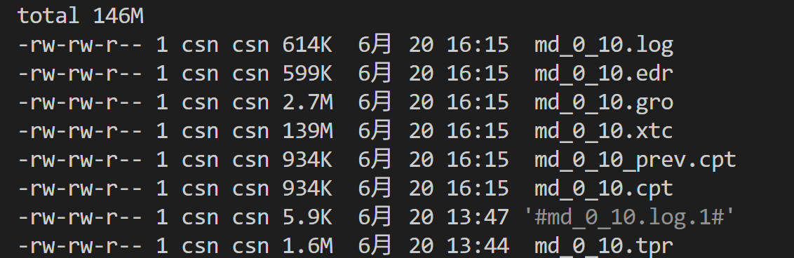
8,Analysis 模拟后分析
Correcting for Periodicity Effects 周期性效应校正
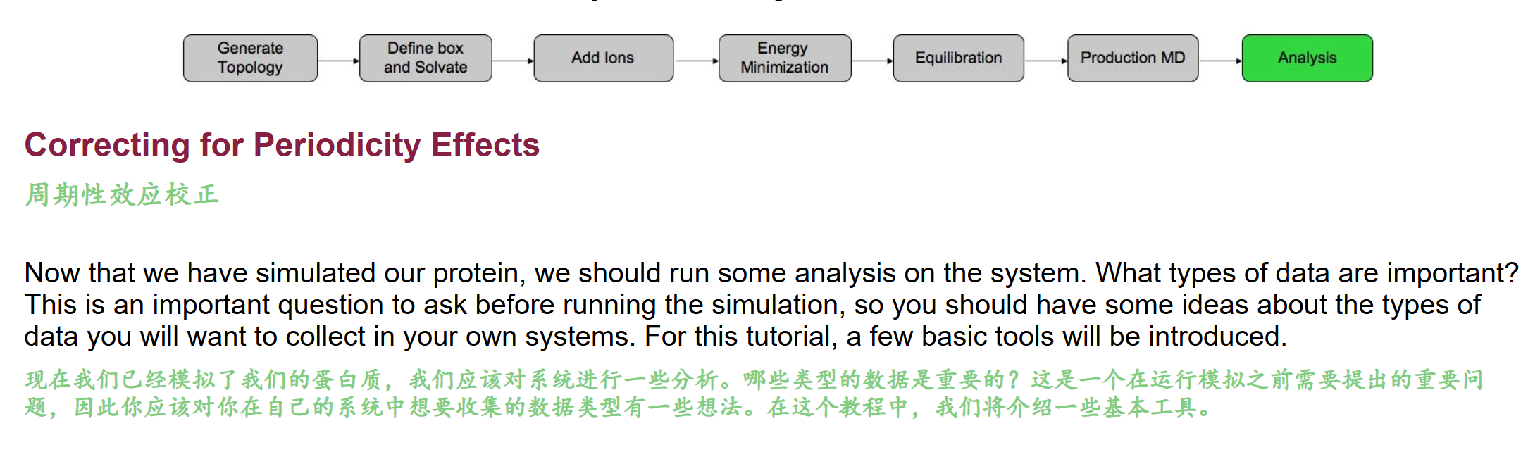
因为下面需要用到gmx trjconv这个工具,所以我们同样进行分析:
理论上trjconv是GROMACS 轨迹后处理基础万能工具,所有可视化、结构分析前几乎必用,核心解决周期性边界 PBC 带来的分子断裂、距离计算失真问题,同时支持格式转换、原子筛选、抽帧、结构对齐
python
gmx trjconv
gmx help trjconv
文档如下
python
SYNOPSIS

gmx trjconv [-f [<.xtc/.trr/...>]] [-s [<.tpr/.gro/...>]] [-n [<.ndx>]]
            [-fr [<.ndx>]] [-sub [<.ndx>]] [-drop [<.xvg>]]
            [-o [<.xtc/.trr/...>]] [-b <time>] [-e <time>] [-tu <enum>]
            [-[no]w] [-xvg <enum>] [-skip <int>] [-dt <time>] [-[no]round]
            [-dump <time>] [-t0 <time>] [-timestep <time>] [-pbc <enum>]
            [-ur <enum>] [-[no]center] [-boxcenter <enum>] [-box <vector>]
            [-trans <vector>] [-shift <vector>] [-fit <enum>] [-ndec <int>]
            [-[no]vel] [-[no]force] [-trunc <time>] [-exec <string>]
            [-split <time>] [-[no]sep] [-nzero <int>] [-dropunder <real>]
            [-dropover <real>] [-[no]conect]

DESCRIPTION

gmx trjconv can convert trajectory files in many ways:

* from one format to another
* select a subset of atoms
* change the periodicity representation
* keep multimeric molecules together
* center atoms in the box
* fit atoms to reference structure
* reduce the number of frames
* change the timestamps of the frames (-t0 and -timestep)
* select frames within a certain range of a quantity given in an .xvg file.

The option to write subtrajectories (-sub) based on the information obtained
from cluster analysis has been removed from gmx trjconv and is now part of
[gmx extract-cluster]

gmx trjcat is better suited for concatenating multiple trajectory files.

The following formats are supported for input and output: .xtc, .trr, .gro,
.g96, .pdb and .tng. The file formats are detected from the file extension.
The precision of the .xtc output is taken from the input file for .xtc, .gro
and .pdb, and from the -ndec option for other input formats. The precision is
always taken from -ndec, when this option is set. All other formats have fixed
precision. .trr output can be single or double precision, depending on the
precision of the gmx trjconv binary. Note that velocities are only supported
in .trr, .tng, .gro and .g96 files.

Option -sep can be used to write every frame to a separate .gro, .g96 or .pdb
file. By default, all frames all written to one file. .pdb files with all
frames concatenated can be viewed with rasmol -nmrpdb.

It is possible to select part of your trajectory and write it out to a new
trajectory file in order to save disk space, e.g. for leaving out the water
from a trajectory of a protein in water. ALWAYS put the original trajectory on
tape! We recommend to use the portable .xtc format for your analysis to save
disk space and to have portable files. When writing .tng output the file will
contain one molecule type of the correct count if the selection name matches
the molecule name and the selected atoms match all atoms of that molecule.
Otherwise the whole selection will be treated as one single molecule
containing all the selected atoms.

There are two options for fitting the trajectory to a reference either for
essential dynamics analysis, etc. The first option is just plain fitting to a
reference structure in the structure file. The second option is a progressive
fit in which the first timeframe is fitted to the reference structure in the
structure file to obtain and each subsequent timeframe is fitted to the
previously fitted structure. This way a continuous trajectory is generated,
which might not be the case when using the regular fit method, e.g. when your
protein undergoes large conformational transitions.

Option -pbc sets the type of periodic boundary condition treatment:

 * mol puts the center of mass of molecules in the box, and requires a run
   input file to be supplied with -s.
 * res puts the center of mass of residues in the box.
 * atom puts all the atoms in the box.
 * nojump checks if atoms jump across the box and then puts them back. This
   has the effect that all molecules will remain whole (provided they were
   whole in the initial conformation). Note that this ensures a continuous
   trajectory but molecules may diffuse out of the box. The starting
   configuration for this procedure is taken from the structure file, if one
   is supplied, otherwise it is the first frame.
 * cluster clusters all the atoms in the selected index such that they are all
   closest to the center of mass of the cluster, which is iteratively updated.
   Note that this will only give meaningful results if you in fact have a
   cluster. Luckily that can be checked afterwards using a trajectory viewer.
   Note also that if your molecules are broken this will not work either.
 * whole only makes broken molecules whole.

Option -ur sets the unit cell representation for options mol, res and atom of
-pbc. All three options give different results for triclinic boxes and
identical results for rectangular boxes. rect is the ordinary brick shape.
tric is the triclinic unit cell. compact puts all atoms at the closest
distance from the center of the box. This can be useful for visualizing e.g.
truncated octahedra or rhombic dodecahedra. The center for options tric and
compact is tric (see below), unless the option -boxcenter is set differently.

Option -center centers the system in the box. The user can select the group
which is used to determine the geometrical center. Option -boxcenter sets the
location of the center of the box for options -pbc and -center. The center
options are: tric: half of the sum of the box vectors, rect: half of the box
diagonal, zero: zero. Use option -pbc mol in addition to -center when you want
all molecules in the box after the centering.

Option -box sets the size of the new box. This option only works for leading
dimensions and is thus generally only useful for rectangular boxes. If you
want to modify only some of the dimensions, e.g. when reading from a
trajectory, you can use -1 for those dimensions that should stay the same It
is not always possible to use combinations of -pbc, -fit, -ur and -center to
do exactly what you want in one call to gmx trjconv. Consider using multiple
calls, and check out the GROMACS website for suggestions.

With -dt, it is possible to reduce the number of frames in the output. This
option relies on the accuracy of the times in your input trajectory, so if
these are inaccurate use the -timestep option to modify the time (this can be
done simultaneously). For making smooth movies, the program gmx filter can
reduce the number of frames while using low-pass frequency filtering, this
reduces aliasing of high frequency motions.

Using -trunc gmx trjconv can truncate .trr in place, i.e. without copying the
file. This is useful when a run has crashed during disk I/O (i.e. full disk),
or when two contiguous trajectories must be concatenated without having double
frames.

Option -dump can be used to extract a frame at or near one specific time from
your trajectory. If the frames in the trajectory are not in temporal order,
the result is unspecified.

Option -drop reads an .xvg file with times and values. When options -dropunder
and/or -dropover are set, frames with a value below and above the value of the
respective options will not be written.

OPTIONS

Options to specify input files:

 -f      [<.xtc/.trr/...>]  (traj.xtc)
           Trajectory: xtc trr cpt gro g96 pdb tng
 -s      [<.tpr/.gro/...>]  (topol.tpr)      (Opt.)
           Structure+mass(db): tpr gro g96 pdb brk ent
 -n      [<.ndx>]           (index.ndx)      (Opt.)
           Index file
 -fr     [<.ndx>]           (frames.ndx)     (Opt.)
           Index file
 -sub    [<.ndx>]           (cluster.ndx)    (Opt.)
           Index file
 -drop   [<.xvg>]           (drop.xvg)       (Opt.)
           xvgr/xmgr file

Options to specify output files:

 -o      [<.xtc/.trr/...>]  (trajout.xtc)
           Trajectory: xtc trr gro g96 pdb tng

Other options:

 -b      <time>             (0)
           Time of first frame to read from trajectory (default unit ps)
 -e      <time>             (0)
           Time of last frame to read from trajectory (default unit ps)
 -tu     <enum>             (ps)
           Unit for time values: fs, ps, ns, us, ms, s
 -[no]w                     (no)
           View output .xvg, .xpm, .eps and .pdb files
 -xvg    <enum>             (xmgrace)
           xvg plot formatting: xmgrace, xmgr, none
 -skip   <int>              (1)
           Only write every nr-th frame
 -dt     <time>             (0)
           Only write frame when t MOD dt = first time (ps)
 -[no]round                 (no)
           Round measurements to nearest picosecond
 -dump   <time>             (-1)
           Dump frame nearest specified time (ps)
 -t0     <time>             (0)
           Starting time (ps) (default: don't change)
 -timestep <time>           (0)
           Change time step between input frames (ps)
 -pbc    <enum>             (none)
           PBC treatment (see help text for full description): none, mol, res,
           atom, nojump, cluster, whole
 -ur     <enum>             (rect)
           Unit-cell representation: rect, tric, compact
 -[no]center                (no)
           Center atoms in box
 -boxcenter <enum>          (tric)
           Center for -pbc and -center: tric, rect, zero
 -box    <vector>           (0 0 0)
           Size for new cubic box (default: read from input)
 -trans  <vector>           (0 0 0)
           All coordinates will be translated by trans. This can
           advantageously be combined with -pbc mol -ur compact.
 -shift  <vector>           (0 0 0)
           All coordinates will be shifted by framenr*shift
 -fit    <enum>             (none)
           Fit molecule to ref structure in the structure file: none,
           rot+trans, rotxy+transxy, translation, transxy, progressive
 -ndec   <int>              (3)
           Number of decimal places to write to .xtc output
 -[no]vel                   (yes)
           Read and write velocities if possible
 -[no]force                 (no)
           Read and write forces if possible
 -trunc  <time>             (-1)
           Truncate input trajectory file after this time (ps)
 -exec   <string>
           Execute command for every output frame with the frame number as
           argument
 -split  <time>             (0)
           Start writing new file when t MOD split = first time (ps)
 -[no]sep                   (no)
           Write each frame to a separate .gro, .g96 or .pdb file
 -nzero  <int>              (0)
           If the -sep flag is set, use these many digits for the file numbers
           and prepend zeros as needed
 -dropunder <real>          (0)
           Drop all frames below this value
 -dropover <real>           (0)
           Drop all frames above this value
 -[no]conect                (no)
           Add CONECT PDB records when writing .pdb files. Useful for
           visualization of non-standard molecules, e.g. coarse grained ones.
           Can only be done when a topology (tpr) file is present
python
# ====================== 第一部分:SYNOPSIS 命令行参数总览释义 ======================
# 输入类参数(读取文件)
# -f:输入轨迹 xtc/trr/cpt/gro/pdb/tng,必选,原始模拟轨迹
# -s:拓扑结构文件 tpr/gro,关键!做PBC校正、居中、拟合、分子完整化必须带-s(含质量、残基、分子拓扑信息)
# -n:索引ndx,自定义原子组(蛋白/水/配体/核酸分组)
# -fr:帧索引文件,按指定帧列表提取
# -sub:旧版聚类分轨迹功能已移除,改用 gmx extract-cluster
# -drop:xvg数据文件,根据数值阈值筛帧(RMSD/RMSF大于/小于某值丢弃帧)

# 输出类参数(生成新轨迹)
# -o:输出校正后轨迹,推荐xtc(高压缩、省空间、通用);trr带速度/力,体积大
# 时间区间控制
# -b:起始时间ps,截取轨迹前段
# -e:终止时间ps,截取轨迹后段
# -tu:时间单位 fs/ps/ns,统一切换时间刻度
# 抽帧降采样
# -skip N:每N帧输出1帧(-skip 10=只存第0,10,20...帧)
# -dt X:仅输出 t % X == 首帧时间 的帧,均匀时间间隔抽帧,比-skip更稳定
# 单帧提取
# -dump time:提取最接近指定时间的单帧pdb/gro,用于截图、初始构象
# 时间戳修改
# -t0:重置轨迹起始时间
# -timestep:强制修改帧间时间步长,修复模拟时间错乱轨迹

# 核心周期性PBC校正模块(全文最重点,对应教程周期性校正)
# -pbc <mode> 周期性重构模式(解决分子跨盒断裂、跳跃问题)
# 1. none:不做任何PBC处理,原始轨迹直接输出
# 2. atom:把所有原子拉回盒内,会把完整分子拆碎(蛋白跨盒直接两半,可视化灾难)
# 3. res:以残基质心为单位放回盒子,适合多肽短链,长蛋白仍易断裂
# 4. mol:以完整分子质心为单位重构(蛋白质整体算一个分子,最常用!教程命令核心参数)
#    硬性依赖-s tpr,程序依靠拓扑识别完整分子,保证蛋白不会被拆断
# 5. whole:仅修复断裂分子,不整体移入盒中心,适合仅修复不居中场景
# 6. nojump:消除原子跨盒跳跃,分子保持连续,但分子可能飘出盒子外,适合长时间扩散分析
# 7. cluster:把所选原子簇收拢到簇质心,仅适合单团聚集体系(蛋白+配体复合物)

# -ur 晶胞显示模式(配合-pbc mol/res/atom使用)
# rect:标准长方体盒子(最常用)
# tric:三斜晶胞原生形态
# compact:将分子摆到离盒子中心最近位置,可视化截断八面体、菱形十二面体盒子

# 居中操作 -[no]center(教程命令第二个核心参数)
# -center:将指定原子组几何中心放到盒子中心,执行时交互选择居中组(教程选1 Protein)
# -boxcenter:定义盒子中心点基准 tric/rect/zero,默认tric
# -trans / -shift:整体坐标平移,微调分子位置,辅助可视化

# 结构拟合 -fit(消除整体平动转动,RMSD分析必备)
# rot+trans:整体旋转+平移对齐参考构象(tpr内初始结构)
# progressive:渐进拟合,每一帧对齐上一帧,适合大幅构象变化蛋白(避免构象跳变断层)

# 格式、精度、拆分输出
# -ndec:xtc坐标保留小数位数,默认3,精度需求高可调4/5
# -[no]vel / -[no]force:是否保留速度、受力,xtc不存速度,trr才支持
# -split X:每隔X ps切分一个独立轨迹文件
# -sep:每一帧单独输出pdb/gro,搭配-nzero补零命名 frame_0001.pdb
# -trunc:原地截断trr文件,磁盘写崩、重复帧拼接修复专用
# -conect:pdb输出添加化学键记录,粗粒化、配体可视化必备,需要-s拓扑文件

# ====================== 第二部分 DESCRIPTION 功能总述核心解读 ======================
# trjconv 本质:轨迹后处理万能转换工具,7大核心用途
# 1. 轨迹格式互转:xtc/trr/gro/pdb/tng 任意互转
# 2. 原子筛选:通过-n ndx只保留蛋白/核酸/配体,剔除水、离子压缩文件体积
# 3. PBC周期性重构(教程核心场景):修复分子跨盒断裂、原子跳跃
# 4. 居中/平移/拟合:对齐蛋白、消除整体运动,用于可视化+RMSD/RMSF分析
# 5. 轨迹裁剪降采样:截取时间区间、均匀抽帧,减少分析计算量
# 6. 时间戳修正:修复模拟中断、步长错乱的轨迹时间轴
# 7. 按xvg数值筛帧:自动丢弃高RMSD异常帧,筛选稳定构象段

# 关键补充文档提示
# 1. 多轨迹拼接不用trjconv,专用工具 gmx trjcat
# 2. -sub聚类分轨迹功能已移除,更换 gmx extract-cluster
# 3. xtc优势:无损压缩、体积极小、跨平台;trr体积大,仅需速度/受力时使用
# 4. 平滑动画降噪不要用dt/skip抽帧,专用 gmx filter 低通滤波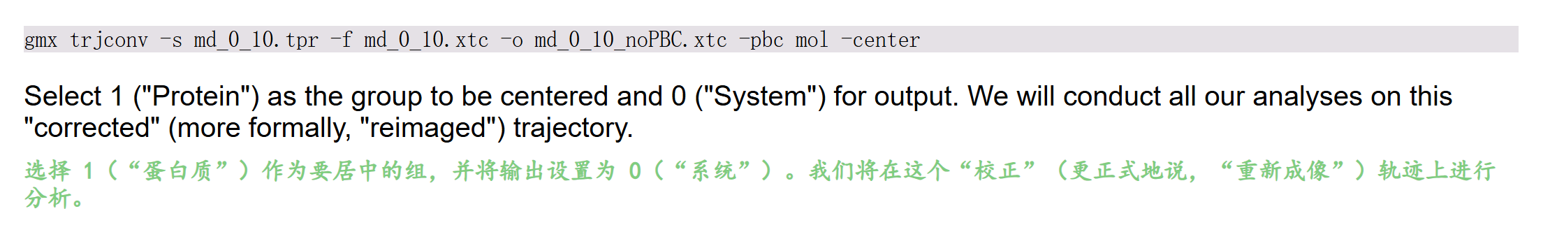
执行命令:
python
gmx trjconv -s md_0_10.tpr -f md_0_10.xtc -o md_0_10_noPBC.xtc -pbc mol -center- -s md_0_10.tpr:必须传入拓扑,程序识别蛋白质为完整分子,实现-pbc mol整分子重构
- -f md_0_10.xtc:原始模拟轨迹,存在蛋白跨晶盒断裂、原子跳变问题
- -o md_0_10_noPBC.xtc:输出校正后无周期性断裂的轨迹(reimaged轨迹)
- -pbc mol:核心校正逻辑------以完整分子为单位,把整个蛋白质放回盒子,杜绝分子拆成两半
- -center:开启居中,交互选择 Protein(组1)作为居中参照物,整个蛋白落在盒子几何中心
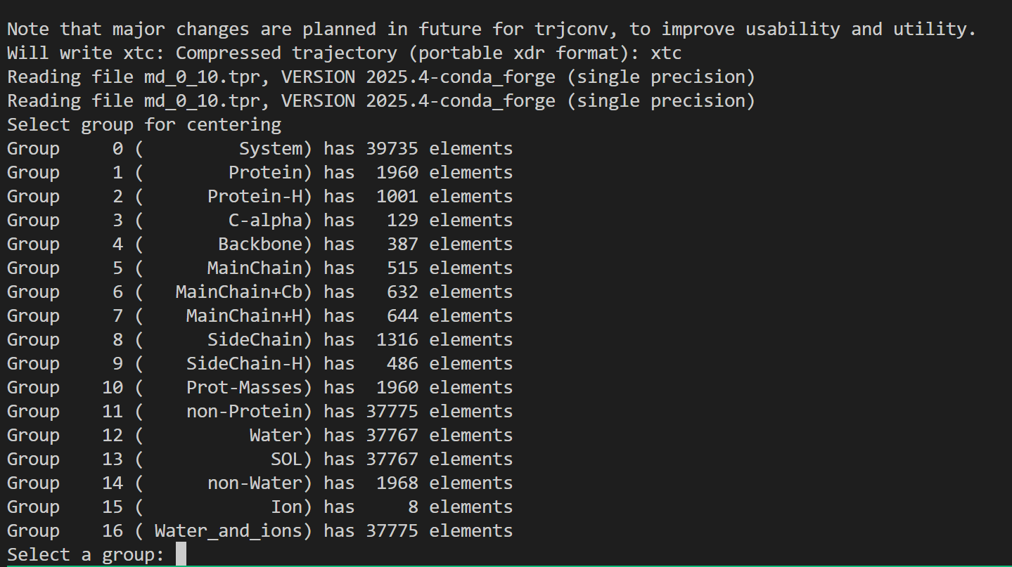
我们选择以目标蛋白质分子为中心,选1
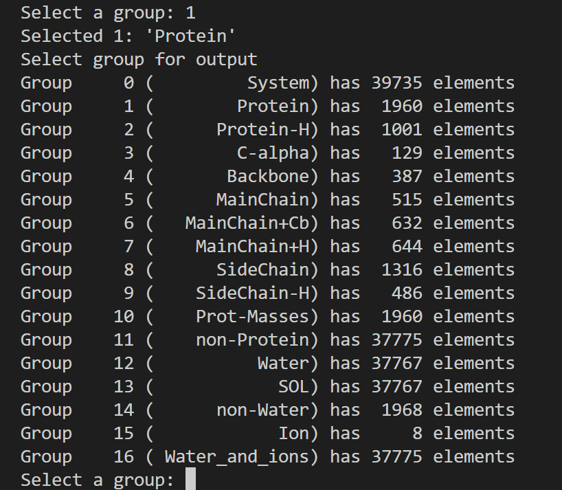
然后输出的话还是以整个体系,选0;
输出日志如下
python
Executable:   /home/csn/program/miniconda3/envs/gromacs/bin.AVX2_256/gmx
Data prefix:  /home/csn/program/miniconda3/envs/gromacs
Working dir:  /mnt/sdb/zht/project/tf-dna-md/files/structure/test
Command line:
  gmx trjconv -s md_0_10.tpr -f md_0_10.xtc -o md_0_10_noPBC.xtc -pbc mol -center

Note that major changes are planned in future for trjconv, to improve usability and utility.
Will write xtc: Compressed trajectory (portable xdr format): xtc
Reading file md_0_10.tpr, VERSION 2025.4-conda_forge (single precision)
Reading file md_0_10.tpr, VERSION 2025.4-conda_forge (single precision)
Select group for centering
Group     0 (         System) has 39735 elements
Group     1 (        Protein) has  1960 elements
Group     2 (      Protein-H) has  1001 elements
Group     3 (        C-alpha) has   129 elements
Group     4 (       Backbone) has   387 elements
Group     5 (      MainChain) has   515 elements
Group     6 (   MainChain+Cb) has   632 elements
Group     7 (    MainChain+H) has   644 elements
Group     8 (      SideChain) has  1316 elements
Group     9 (    SideChain-H) has   486 elements
Group    10 (    Prot-Masses) has  1960 elements
Group    11 (    non-Protein) has 37775 elements
Group    12 (          Water) has 37767 elements
Group    13 (            SOL) has 37767 elements
Group    14 (      non-Water) has  1968 elements
Group    15 (            Ion) has     8 elements
Group    16 ( Water_and_ions) has 37775 elements
Select a group: 1
Selected 1: 'Protein'
Select group for output
Group     0 (         System) has 39735 elements
Group     1 (        Protein) has  1960 elements
Group     2 (      Protein-H) has  1001 elements
Group     3 (        C-alpha) has   129 elements
Group     4 (       Backbone) has   387 elements
Group     5 (      MainChain) has   515 elements
Group     6 (   MainChain+Cb) has   632 elements
Group     7 (    MainChain+H) has   644 elements
Group     8 (      SideChain) has  1316 elements
Group     9 (    SideChain-H) has   486 elements
Group    10 (    Prot-Masses) has  1960 elements
Group    11 (    non-Protein) has 37775 elements
Group    12 (          Water) has 37767 elements
Group    13 (            SOL) has 37767 elements
Group    14 (      non-Water) has  1968 elements
Group    15 (            Ion) has     8 elements
Group    16 ( Water_and_ions) has 37775 elements
Select a group: 0
Selected 0: 'System'
Reading frame       0 time    0.000
Precision of md_0_10.xtc is 0.001 (nm)
Using output precision of 0.001 (nm)
Last frame       1000 time 10000.000    ->  frame    999 time 9990.000
 ->  frame   1000 time 10000.000
Last written: frame   1000 time 10000.000
一并作中文注释
python
# ===================== 运行环境信息 =====================
Executable:   /home/csn/program/miniconda3/envs/gromacs/bin.AVX2_256/gmx
// 当前调用的GROMACS可执行文件路径;基于conda虚拟环境,启用AVX2 256位CPU加速指令集
Data prefix:  /home/csn/program/miniconda3/envs/gromacs
// GROMACS程序库、力场文件、拓扑模板的根目录
Working dir:  /mnt/sdb/zht/project/tf-dna-md/files/structure/test
// 命令执行的工作目录,所有输入输出文件均在此路径下查找/生成

# ===================== 执行命令 =====================
Command line:
  gmx trjconv -s md_0_10.tpr -f md_0_10.xtc -o md_0_10_noPBC.xtc -pbc mol -center
// trjconv轨迹处理工具核心参数回顾
// -s 输入拓扑运行文件;-f 原始模拟轨迹;-o 校正后无PBC断裂轨迹
// -center 体系居中;-pbc mol 按完整分子修复周期性边界撕裂

# ===================== 程序前置提示 =====================
Note that major changes are planned in future for trjconv, to improve usability and utility.
// GROMACS官方提示:未来版本会重构trjconv工具,优化使用逻辑
Will write xtc: Compressed trajectory (portable xdr format): xtc
// 指定输出文件格式为xtc:压缩二进制轨迹,体积小、跨软件通用

# ===================== 读取拓扑文件 =====================
Reading file md_0_10.tpr, VERSION 2025.4-conda_forge (single precision)
Reading file md_0_10.tpr, VERSION 2025.4-conda_forge (single precision)
// 读取tpr拓扑文件两次(一次提取分组信息,一次提取盒子、分子拓扑)
// 模拟版本2025.4 conda编译版,单精度浮点计算(常规MD默认)

# ===================== 第一次交互:选择居中参考组 =====================
Select group for centering
// -center 参数触发:选择以哪一组原子为基准平移至盒子中心
Group     0 (         System) has 39735 elements   // 整个体系全部原子
Group     1 (        Protein) has  1960 elements   // 蛋白原子(本次选中)
Group     2 (      Protein-H) has  1001 elements   // 蛋白氢原子
Group     3 (        C-alpha) has   129 elements   // 蛋白CA主链碳原子
Group     4 (       Backbone) has   387 elements   // 蛋白主链原子
Group     5 (      MainChain) has   515 elements
Group     6 (   MainChain+Cb) has   632 elements
Group     7 (    MainChain+H) has   644 elements
Group     8 (      SideChain) has  1316 elements   // 蛋白侧链原子
Group     9 (    SideChain-H) has   486 elements
Group    10 (    Prot-Masses) has  1960 elements
Group    11 (    non-Protein) has 37775 elements   // 水+离子全部溶剂
Group    12 (          Water) has 37767 elements  // 水分子
Group    13 (            SOL) has 37767 elements  // SOL等价于Water
Group    14 (      non-Water) has  1968 elements  // 蛋白+离子
Group    15 (            Ion) has     8 elements   // 体系中和离子
Group    16 ( Water_and_ions) has 37775 elements   // 水+离子
Select a group: 1
Selected 1: 'Protein'
// 选择1号Protein组作为居中基准:每一帧把蛋白平移到盒子几何中心
// 优势:避免蛋白跨盒子撕裂,后续PBC校正效果最优;适合蛋白-溶剂体系

# ===================== 第二次交互:选择输出轨迹包含原子组 =====================
Select group for output
// 选择最终输出xtc文件里保留哪些原子,分组列表同上不再重复注释
Select a group: 0
Selected 0: 'System'
// 选择0号System全体系输出:校正后轨迹同时保留蛋白、水、离子所有原子
// 若只输出蛋白可填1,后续可视化RMSD只需蛋白可减小文件体积;这里保留完整体系

# ===================== 轨迹逐帧处理日志 =====================
Reading frame       0 time    0.000
// 开始读取第0帧,模拟时间0 ns(模拟初始结构)
Precision of md_0_10.xtc is 0.001 (nm)
Using output precision of 0.001 (nm)
// 原始xtc坐标存储精度0.001 nm,输出轨迹沿用同等精度,不损失坐标细节
Last frame       1000 time 10000.000    ->  frame    999 time 9990.000
 ->  frame   1000 time 10000.000
// 总帧数1001帧(0~1000),总模拟时长10000 ps = 10 ns;中间打印进度提示
Last written: frame   1000 time 10000.000
// 关键收尾标识:全部1001帧校正完成,md_0_10_noPBC.xtc完整写入磁盘
// 无报错、无截断,轨迹校正流程执行成功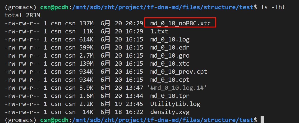
为什么必须做周期性校正?
- MD模拟采用周期性边界条件,蛋白扩散时一半在盒左、一半在盒右,VMD可视化会出现断裂;
- RMSD、RMSF、回旋半径等分析工具计算原子距离时,跨盒原子距离会计算错误,结果完全失真;
- 经过-pbc mol -center重构后的轨迹,所有后续分析(RMSD/RMSF/氢键/二面角)才能得到正确数据。
- 一些PBC参数校正优先级
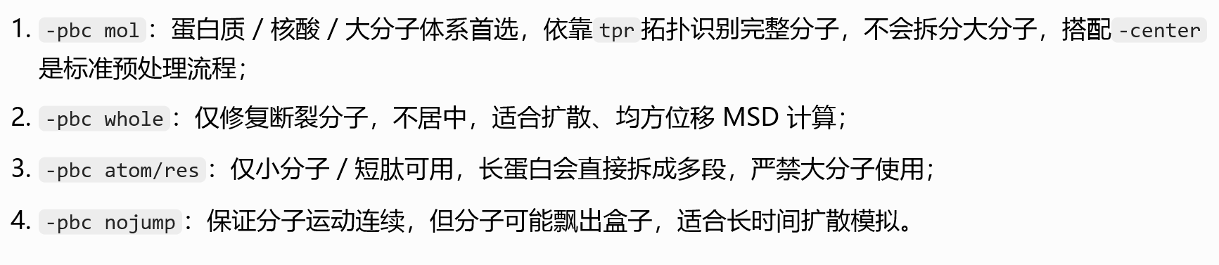
1. 基础输入输出文件类
-s md_0_10.tpr
-s:structure/tpr 拓扑运行文件,必须参数- 作用:提供体系完整拓扑、盒子尺寸、原子编号、分子归属、力场信息;做居中、PBC校正都依赖tpr里的盒子与分子定义,轨迹文件xtc不含拓扑信息,不能单独做PBC处理。
-f md_0_10.xtc
-f:input trajectory 输入轨迹- 作用:指定要处理的原始模拟轨迹(压缩型xtc,存储每一帧原子坐标)。
-o md_0_10_noPBC.xtc
-o:output trajectory 输出处理后轨迹- 文件名含义:
noPBC代表消除周期性断层后的轨迹,输出仍为xtc格式。
2. 核心处理功能参数
-center
- 功能:体系居中校正
- 原理:默认把系统中体积最大的分子/复合物平移到模拟盒子几何中心;
- 配套逻辑:先居中再做PBC重整,能大幅减少分子跨盒子断裂问题,否则大分子一半在盒子左、一半在右,校正后依然撕裂。
- 运行时会弹窗让你选择「居中参考组」(常见选 Protein / System)。
-pbc mol
-pbc:周期性边界条件校正模式,mol= per molecule 按分子重整- 作用:修复PBC导致的分子撕裂(模拟中分子跑出盒子会从对面重新进入,轨迹里分子被切成两半);
mol规则:以完整分子为最小单元,把分散在盒子两侧的同一分子全部平移到同一个盒子内,保证每个分子连续完整;
其他可选模式对比:-pbc res:按残基重整(适合多肽/蛋白,极少用)-pbc atom:仅单原子校正,大分子会断链
整条命令整体作用
读取tpr拓扑+原始xtc轨迹:
- 将目标分子居中到盒子中心
- 按完整分子消除周期性边界撕裂
- 输出一条无分子断裂、体系居中的新轨迹
md_0_10_noPBC.xtc,后续RMSD、RMSF、构象可视化都用这条校正后轨迹。
执行后程序会交互两次选择组:
-center:选择居中对象(一般Protein)-pbc:选择校正基准组(一般System/Protein)
总的来说,前面的分析就是:
原始 xtc 轨迹 → gmx trjconv(-pbc mol -center PBC 校正)→ 校正后轨迹 → RMSD/RMSF/ 氢键 / 二面角等分析工具
python
# 场景1:标准周期性校正(教程同款,蛋白-水溶液体系通用)
# gmx trjconv -s topol.tpr -f traj.xtc -o traj_fix.xtc -pbc mol -center
# 选Protein居中,输出System

# 场景2:仅提取蛋白,剔除水离子,同时修复PBC
# gmx trjconv -s topol.tpr -f traj.xtc -o protein_only.xtc -pbc mol -center -n index.ndx

# 场景3:均匀抽帧,每100ps输出一帧减少计算量
# gmx trjconv -s topol.tpr -f traj.xtc -o traj_sample.xtc -pbc mol -center -dt 100

# 场景4:提取5ns单帧用于绘图
# gmx trjconv -s topol.tpr -f traj.xtc -o frame_5ns.pdb -dump 5000

# 场景5:轨迹对齐参考结构(消除整体平动转动,RMSD前置处理)
# gmx trjconv -s topol.tpr -f traj.xtc -o traj_fit.xtc -pbc mol -center -fit rot+trans

# 场景6:只修复分子断裂,不居中,适合扩散系数计算
# gmx trjconv -s topol.tpr -f traj.xtc -o traj_whole.xtc -pbc whole
Root-Mean-Square Deviation 均方根偏差
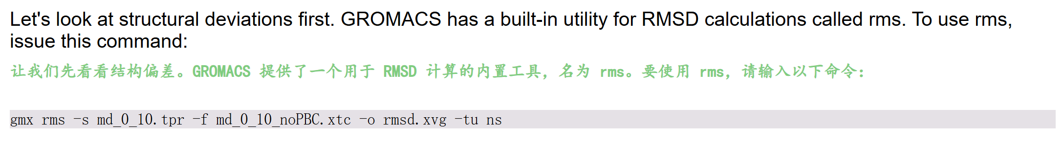
我们看一下这个命令
python
gmx rms
gmx help rms
文档指南如下
python
SYNOPSIS

gmx rms [-s [<.tpr/.gro/...>]] [-f [<.xtc/.trr/...>]]
        [-f2 [<.xtc/.trr/...>]] [-n [<.ndx>]] [-o [<.xvg>]] [-mir [<.xvg>]]
        [-a [<.xvg>]] [-dist [<.xvg>]] [-m [<.xpm>]] [-bin [<.dat>]]
        [-bm [<.xpm>]] [-b <time>] [-e <time>] [-dt <time>] [-tu <enum>]
        [-[no]w] [-xvg <enum>] [-what <enum>] [-[no]pbc] [-fit <enum>]
        [-prev <int>] [-[no]split] [-skip <int>] [-skip2 <int>] [-max <real>]
        [-min <real>] [-bmax <real>] [-bmin <real>] [-[no]mw]
        [-nlevels <int>] [-ng <int>]

DESCRIPTION

gmx rms compares two structures by computing the root mean square deviation
(RMSD), the size-independent rho similarity parameter (rho) or the scaled rho
(rhosc), see Maiorov & Crippen, Proteins 22, 273 (1995). This is selected by
-what.

Each structure from a trajectory (-f) is compared to a reference structure.
The reference structure is taken from the structure file (-s).

With option -mir also a comparison with the mirror image of the reference
structure is calculated. This is useful as a reference for 'significant'
values, see Maiorov & Crippen, Proteins 22, 273 (1995).

Option -prev produces the comparison with a previous frame the specified
number of frames ago.

Option -m produces a matrix in .xpm format of comparison values of each
structure in the trajectory with respect to each other structure. This file
can be visualized with for instance xv and can be converted to postscript with
gmx xpm2ps.

Option -fit controls the least-squares fitting of the structures on top of
each other: complete fit (rotation and translation), translation only, or no
fitting at all.

Option -mw controls whether mass weighting is done or not. If you select the
option (default) and supply a valid .tpr file masses will be taken from there,
otherwise the masses will be deduced from the atommass.dat file in GMXLIB
(deprecated). This is fine for proteins, but not necessarily for other
molecules. You can check whether this happened by turning on the -debug flag
and inspecting the log file.

With -f2, the 'other structures' are taken from a second trajectory, this
generates a comparison matrix of one trajectory versus the other.

Option -bin does a binary dump of the comparison matrix.

Option -bm produces a matrix of average bond angle deviations analogously to
the -m option. Only bonds between atoms in the comparison group are
considered.

OPTIONS

Options to specify input files:

 -s      [<.tpr/.gro/...>]  (topol.tpr)
           Structure+mass(db): tpr gro g96 pdb brk ent
 -f      [<.xtc/.trr/...>]  (traj.xtc)
           Trajectory: xtc trr cpt gro g96 pdb tng
 -f2     [<.xtc/.trr/...>]  (traj.xtc)       (Opt.)
           Trajectory: xtc trr cpt gro g96 pdb tng
 -n      [<.ndx>]           (index.ndx)      (Opt.)
           Index file

Options to specify output files:

 -o      [<.xvg>]           (rmsd.xvg)
           xvgr/xmgr file
 -mir    [<.xvg>]           (rmsdmir.xvg)    (Opt.)
           xvgr/xmgr file
 -a      [<.xvg>]           (avgrp.xvg)      (Opt.)
           xvgr/xmgr file
 -dist   [<.xvg>]           (rmsd-dist.xvg)  (Opt.)
           xvgr/xmgr file
 -m      [<.xpm>]           (rmsd.xpm)       (Opt.)
           X PixMap compatible matrix file
 -bin    [<.dat>]           (rmsd.dat)       (Opt.)
           Generic data file
 -bm     [<.xpm>]           (bond.xpm)       (Opt.)
           X PixMap compatible matrix file

Other options:

 -b      <time>             (0)
           Time of first frame to read from trajectory (default unit ps)
 -e      <time>             (0)
           Time of last frame to read from trajectory (default unit ps)
 -dt     <time>             (0)
           Only use frame when t MOD dt = first time (default unit ps)
 -tu     <enum>             (ps)
           Unit for time values: fs, ps, ns, us, ms, s
 -[no]w                     (no)
           View output .xvg, .xpm, .eps and .pdb files
 -xvg    <enum>             (xmgrace)
           xvg plot formatting: xmgrace, xmgr, none
 -what   <enum>             (rmsd)
           Structural difference measure: rmsd, rho, rhosc
 -[no]pbc                   (yes)
           PBC check
 -fit    <enum>             (rot+trans)
           Fit to reference structure: rot+trans, translation, none
 -prev   <int>              (0)
           Compare with previous frame
 -[no]split                 (no)
           Split graph where time is zero
 -skip   <int>              (1)
           Only write every nr-th frame to matrix
 -skip2  <int>              (1)
           Only write every nr-th frame to matrix
 -max    <real>             (-1)
           Maximum level in comparison matrix
 -min    <real>             (-1)
           Minimum level in comparison matrix
 -bmax   <real>             (-1)
           Maximum level in bond angle matrix
 -bmin   <real>             (-1)
           Minimum level in bond angle matrix
 -[no]mw                    (yes)
           Use mass weighting for superposition
 -nlevels <int>             (80)
           Number of levels in the matrices
 -ng     <int>              (1)
           Number of groups to compute RMS between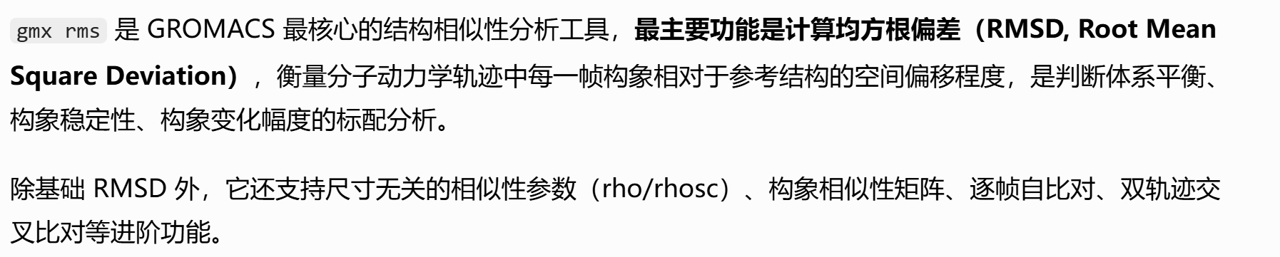
以 -s 指定的结构为参考构象,对 -f 轨迹的每一帧逐一执行「结构叠合 → 偏差计算」,输出对应时间点的偏差值序列。
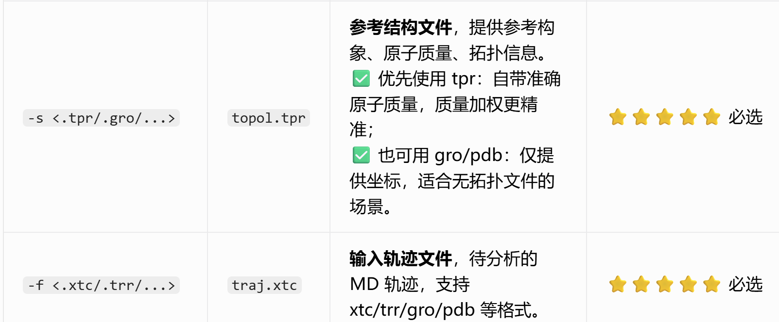
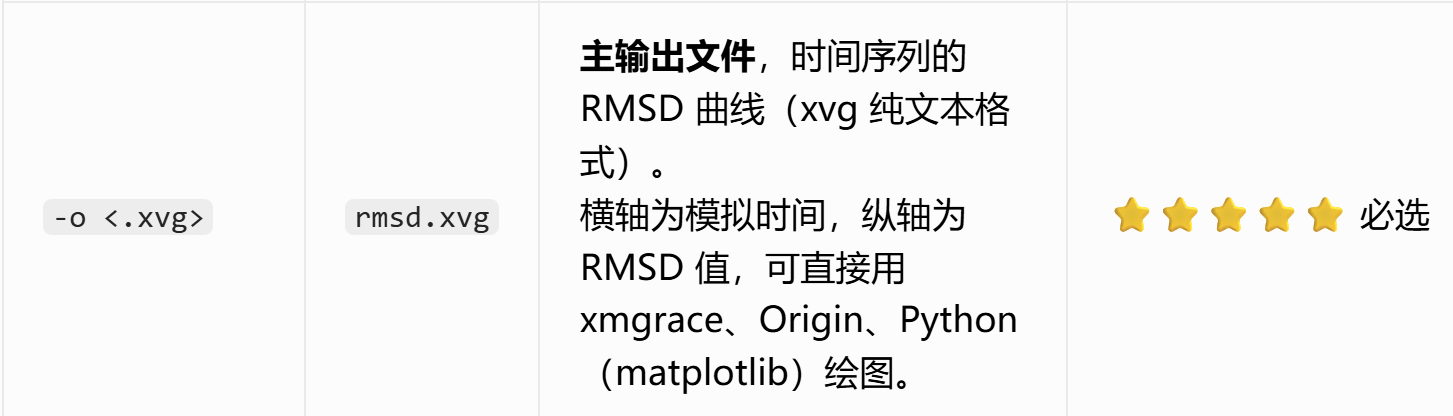
我们执行命令如下
python
gmx rms -s md_0_10.tpr -f md_0_10_noPBC.xtc -o rmsd.xvg -tu ns这里我们按照教程选择主链骨架,
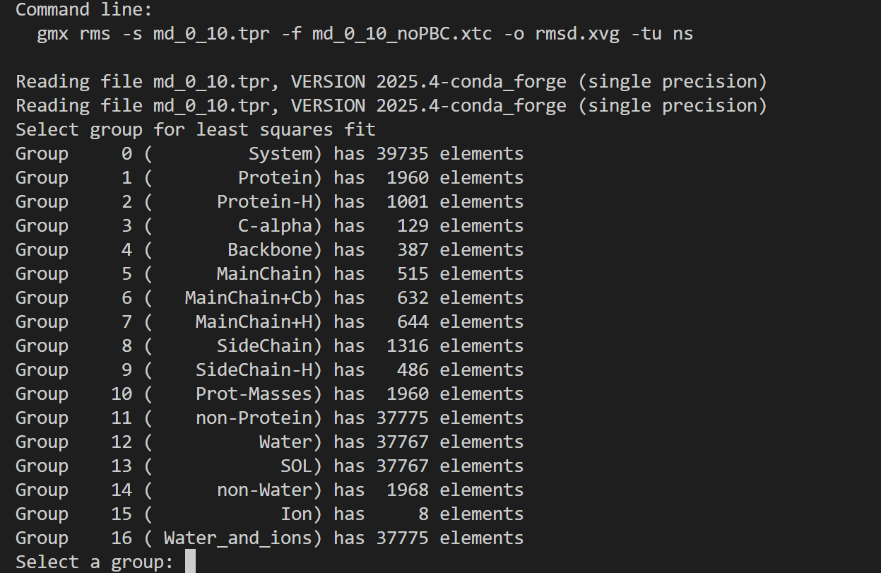
同理RMSD
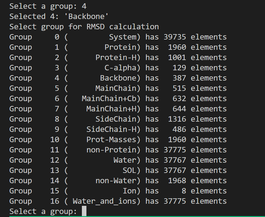
整体运行日志如下
python
Executable:   /home/csn/program/miniconda3/envs/gromacs/bin.AVX2_256/gmx
Data prefix:  /home/csn/program/miniconda3/envs/gromacs
Working dir:  /mnt/sdb/zht/project/tf-dna-md/files/structure/test
Command line:
  gmx rms -s md_0_10.tpr -f md_0_10_noPBC.xtc -o rmsd.xvg -tu ns

Reading file md_0_10.tpr, VERSION 2025.4-conda_forge (single precision)
Reading file md_0_10.tpr, VERSION 2025.4-conda_forge (single precision)
# ⚠️ 最小二乘叠合组选择
# 选择用于全局对齐、消除整体平动旋转的原子组
Select group for least squares fit
Group     0 (         System) has 39735 elements
Group     1 (        Protein) has  1960 elements
Group     2 (      Protein-H) has  1001 elements
Group     3 (        C-alpha) has   129 elements
Group     4 (       Backbone) has   387 elements
Group     5 (      MainChain) has   515 elements
Group     6 (   MainChain+Cb) has   632 elements
Group     7 (    MainChain+H) has   644 elements
Group     8 (      SideChain) has  1316 elements
Group     9 (    SideChain-H) has   486 elements
Group    10 (    Prot-Masses) has  1960 elements
Group    11 (    non-Protein) has 37775 elements
Group    12 (          Water) has 37767 elements
Group    13 (            SOL) has 37767 elements
Group    14 (      non-Water) has  1968 elements
Group    15 (            Ion) has     8 elements
Group    16 ( Water_and_ions) has 37775 elements
Select a group: 4
# 用蛋白主链原子做结构叠合(行业标准操作,避免侧链柔性干扰对齐)
Selected 4: 'Backbone'
Select group for RMSD calculation

# 实际计算RMSD的原子组
Group     0 (         System) has 39735 elements
Group     1 (        Protein) has  1960 elements
Group     2 (      Protein-H) has  1001 elements
Group     3 (        C-alpha) has   129 elements
Group     4 (       Backbone) has   387 elements
Group     5 (      MainChain) has   515 elements
Group     6 (   MainChain+Cb) has   632 elements
Group     7 (    MainChain+H) has   644 elements
Group     8 (      SideChain) has  1316 elements
Group     9 (    SideChain-H) has   486 elements
Group    10 (    Prot-Masses) has  1960 elements
Group    11 (    non-Protein) has 37775 elements
Group    12 (          Water) has 37767 elements
Group    13 (            SOL) has 37767 elements
Group    14 (      non-Water) has  1968 elements
Group    15 (            Ion) has     8 elements
Group    16 ( Water_and_ions) has 37775 elements
Select a group: 4
# 计算蛋白主链自身的RMSD,最常用指标,用来判断蛋白骨架稳定性
Selected 4: 'Backbone'
# 轨迹总帧数0~1000,总模拟时长10 ns
Last frame       1000 time   10.000
教程这里还对前面能量最小化阶段的拓扑结构作为参考进行了RMSD分析
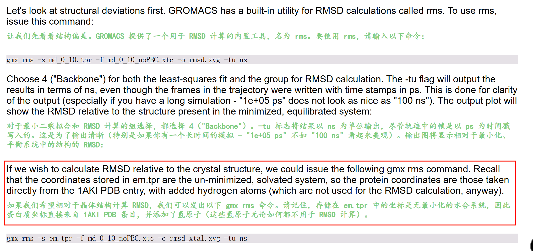
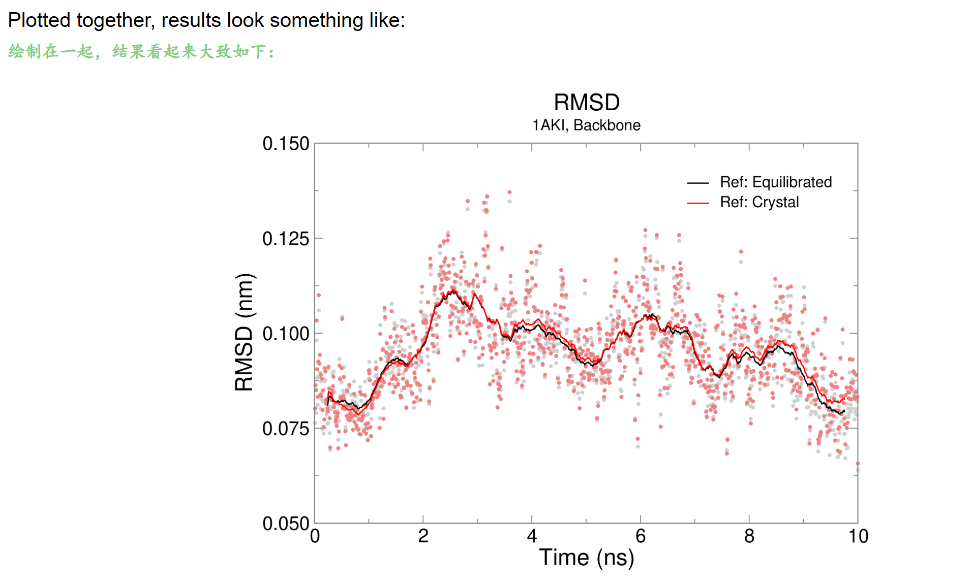
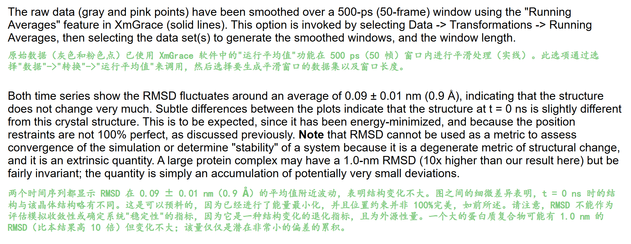
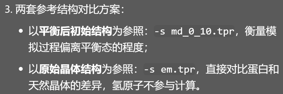
同样的,我们用自己开发的工具来可视化一下这个xvg文件,
依旧是前面说的开发的https://github.com/MaybeBio/gmxplot
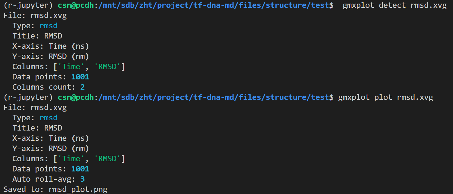
python
# 检测数据类型
gmxplot detect rmsd.xvg
# 绘图
gmxplot plot rmsd.xvg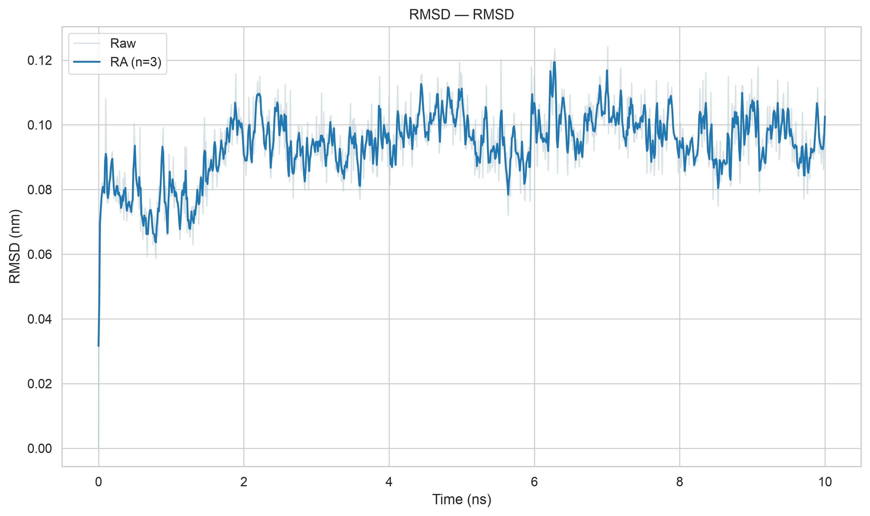
同样对于em阶段的结构,我们也与此处模拟进行了RMSD比对
python
gmx rms -s ../em.tpr -f md_0_10_noPBC.xtc -o rmsd_xtal.xvg -tu ns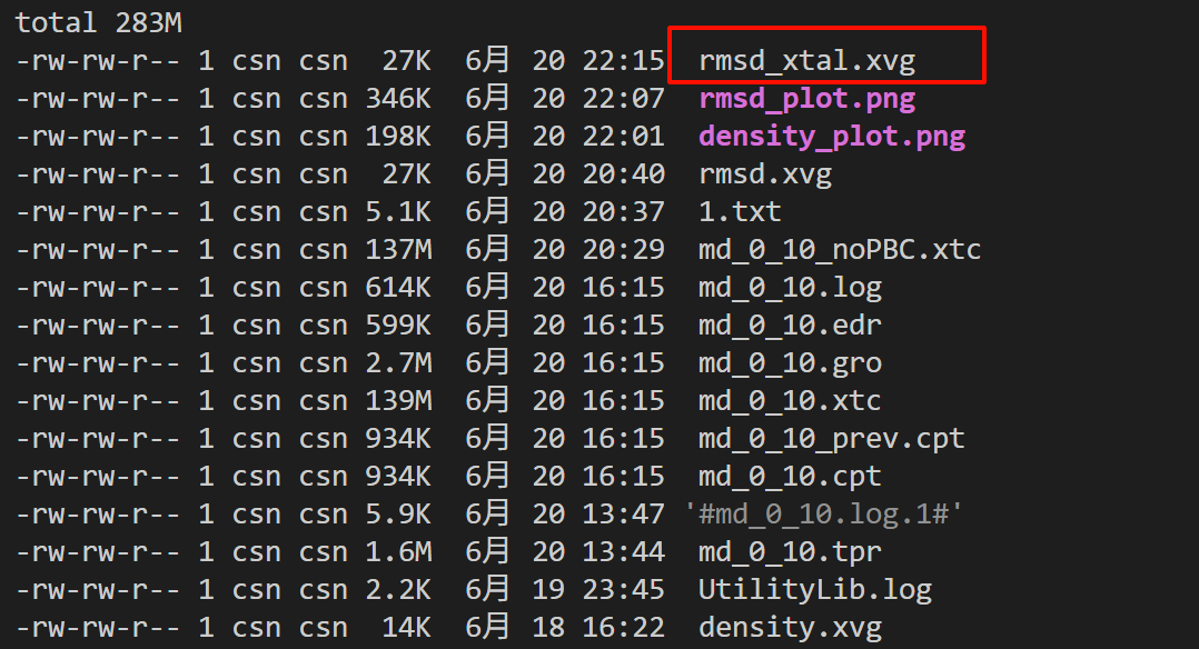
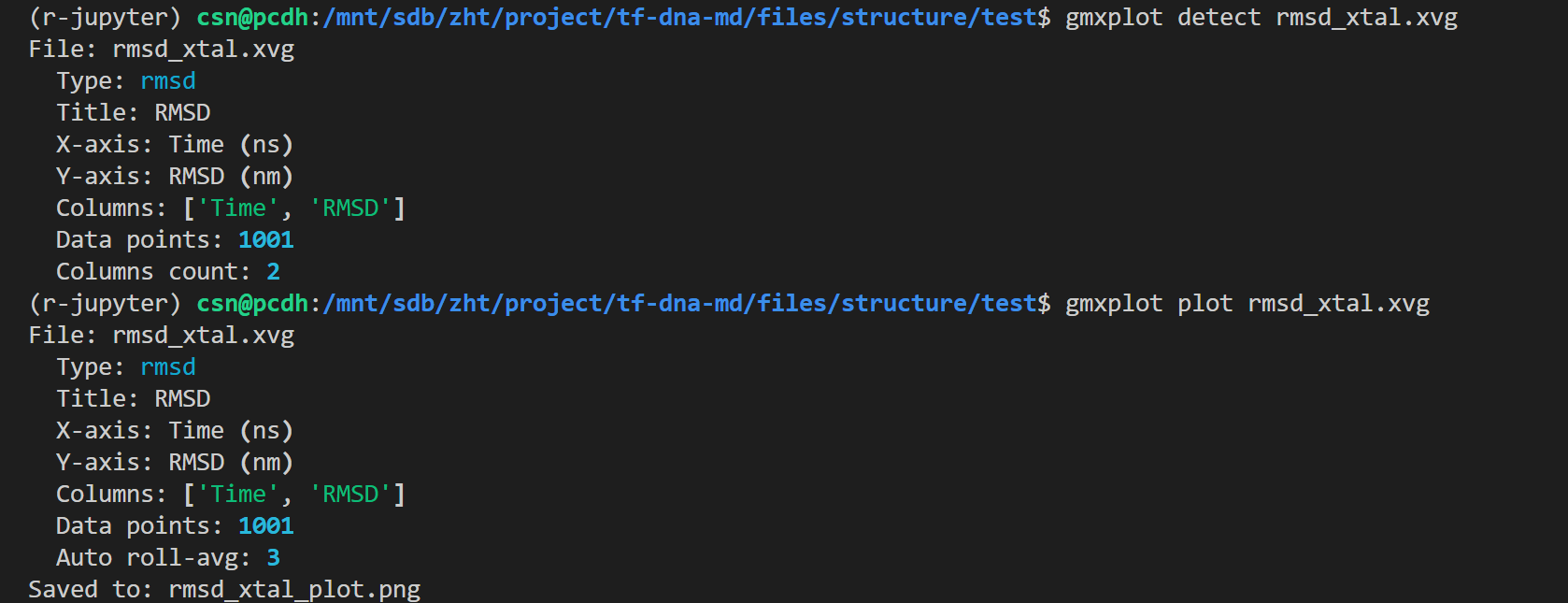
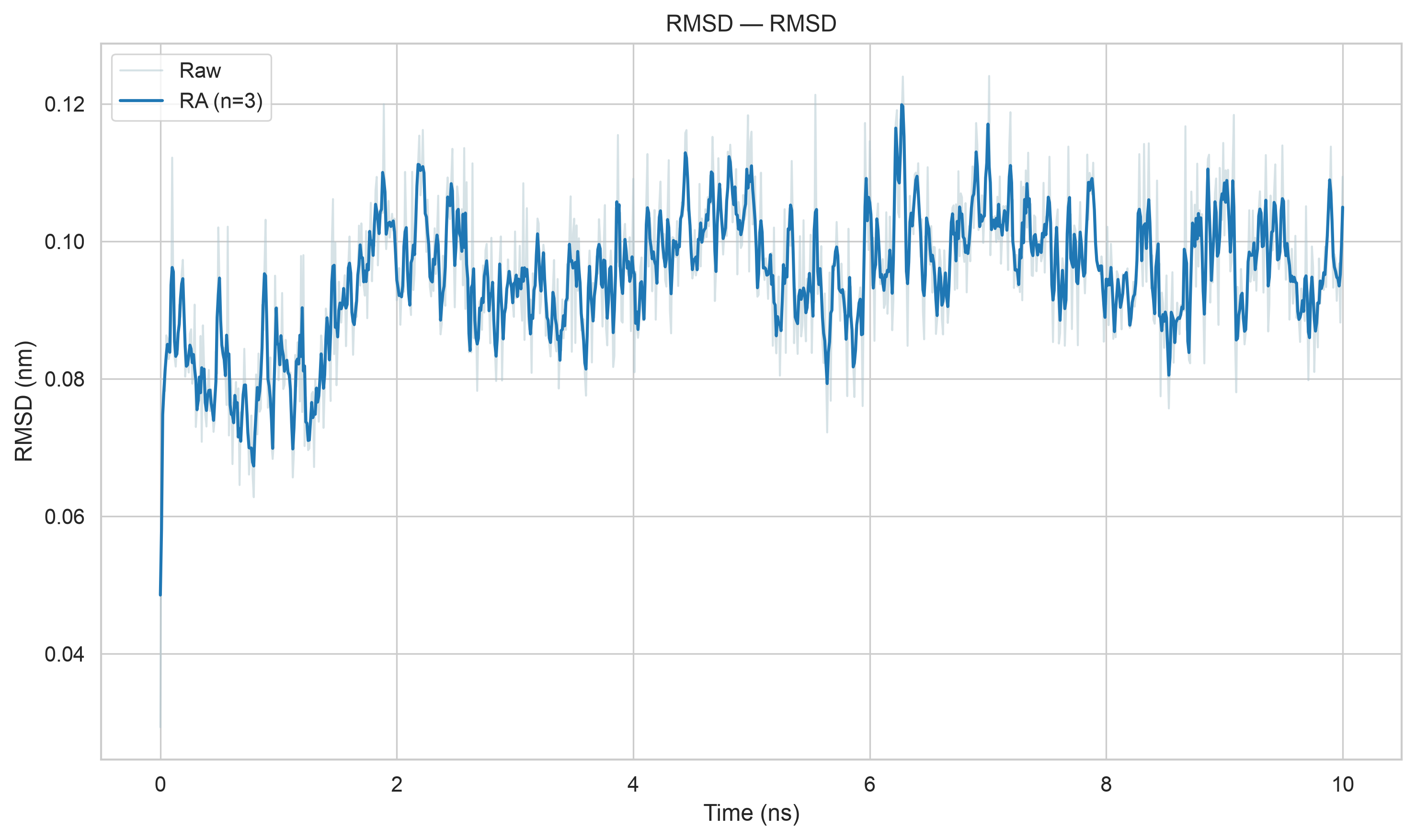
然后两组比较
python
gmxplot compare rmsd_xtal.xvg rmsd.xvg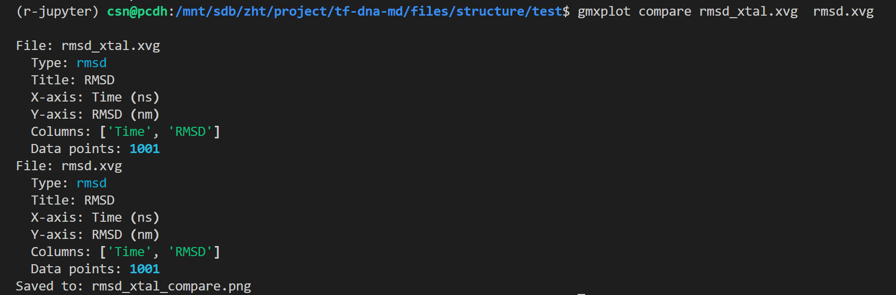
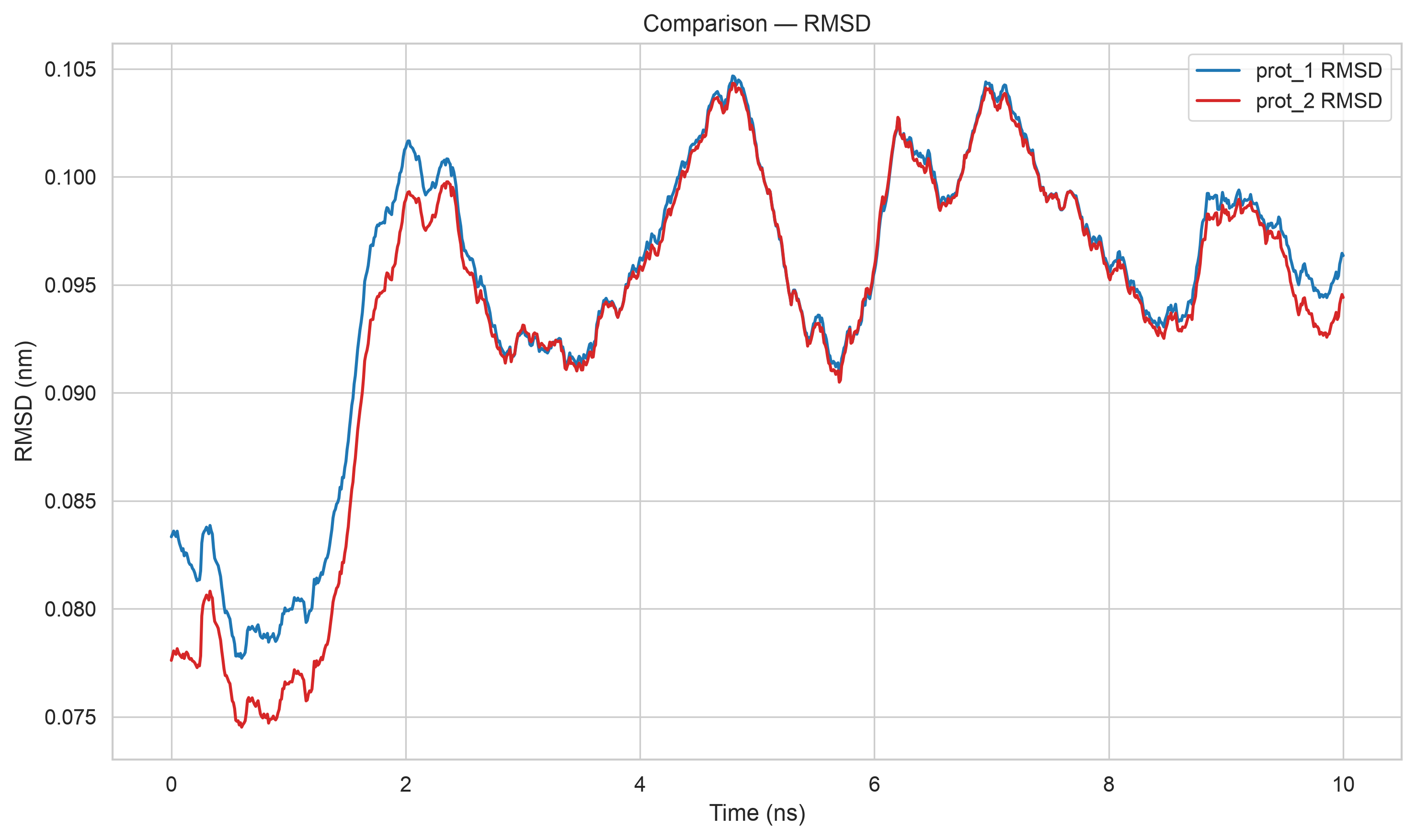
数据略微有差异,这个前面说了,我们的模拟和教程不可能是百分百相似的,
但是效果达到了就行
为什么要做两组RMSD对比:平衡后初始结构 vs 原始晶体结构
一、第一条:-s md_0_10.tpr(平衡完成后的初始结构做参考)
1. 参考结构含义
md_0_10.tpr 是能量最小化+NVT/NPT平衡全部跑完、正式生产MD刚启动时的结构,代表体系已经放松、溶剂盒子、温度压力全部稳定后的构象。
2. 计算目的(看模拟过程内部波动)
- 判断生产模拟是否达到稳定、平衡:
曲线前期快速上升,后期稳定小幅震荡 → 说明体系在模拟前段弛豫完毕,后半段是稳定采样区间; - 只关心模拟过程里蛋白相对于自己平衡态的偏移 :
消除晶体、能量最小化带来的初始构象差异,单纯评价生产MD阶段骨架的柔性波动; - 用来筛选后续分析区间:
比如曲线5 ns后才平稳,后续RMSF、氢键、自由能只取5--10 ns数据,避开未弛豫的前期。
二、第二条:-s em.tpr(能量最小化前,原生晶体结构做参考)
1. 参考结构含义
em.tpr 仅做了溶剂化,还没能量最小化,蛋白原子坐标完全直接取自PDB晶体结构(仅补全氢),代表蛋白天然晶体构象。
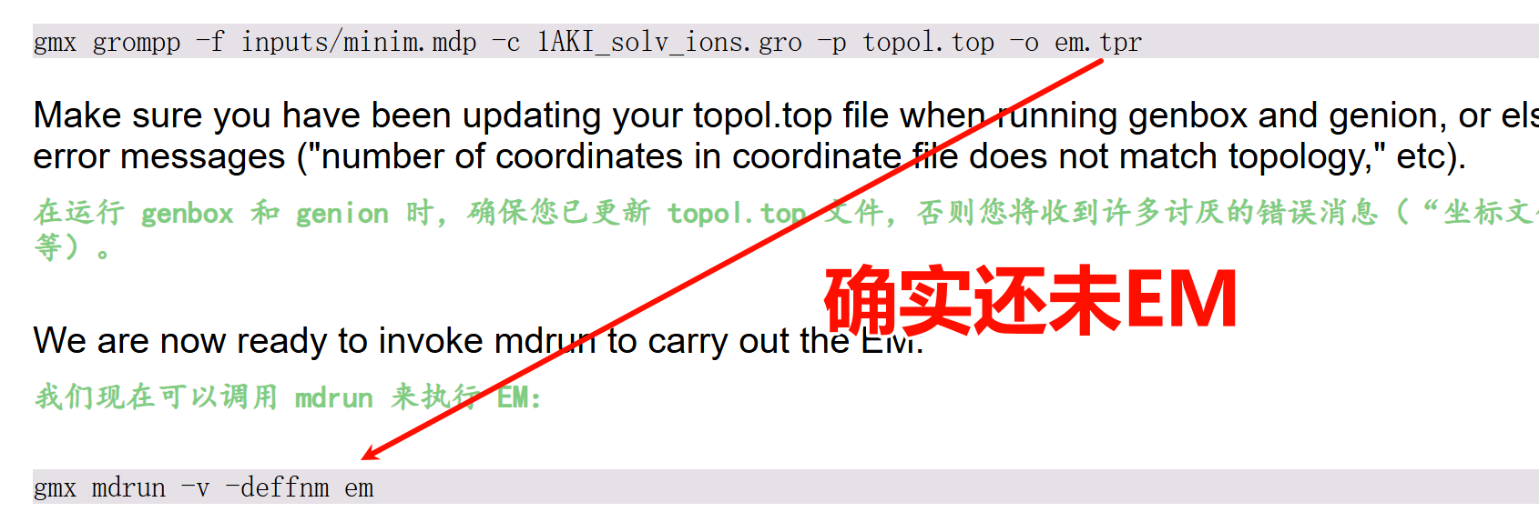
2. 计算目的(看模拟偏离天然晶体的整体程度)
- 评估蛋白在水溶液模拟后,和原生晶体构象的差异大小;
- 回答课题关心的关键问题:
水溶液环境下蛋白骨架是否还能维持晶体天然折叠?RMSD整体很低说明折叠稳定; - 两条曲线会出现固定差值:
t=0时刻两条RMSD不重合,就是因为平衡步骤(最小化+控温控压)已经轻微改变了晶体坐标。
三、两组同时对比的完整逻辑
- 内部稳定性(md_0_10.tpr)
只看生产模拟自身波动,判断采样区间是否平稳,服务于后续动力学定量分析; - 天然构象保留度(em.tpr 晶体)
对比模拟构象与体外晶体结构的差别,解释蛋白在溶液中的构象保持能力,用于论文讨论; - 两者结合才能完整解读:
- 若两条曲线都平稳、数值低:蛋白在水溶液稳定保持天然晶体折叠;
- 晶体参照的RMSD持续走高、平衡参照曲线后期平稳:说明蛋白只是相对于晶体舒展,但模拟内部构象不再大幅变化;
- 原文提到二者均值都在0.09 nm左右小幅波动:
证明即使经过溶剂化、最小化、平衡,蛋白整体骨架和晶体相差很小,折叠结构稳定。
四、两条曲线存在微小差值的原因
- 能量最小化会轻微调整晶体原子坐标,消除原子近距离排斥;
- NVT/NPT平衡阶段去除位置约束、溶剂热运动拉扯蛋白,骨架发生微小弛豫;
- 晶体是低温体外静态结构,模拟是室温水溶液动态环境,天然存在构象差异。
五、总结
- 以平衡态md tpr 为参照:评价生产模拟内部是否稳定,筛选有效采样时间;
- 以未最小化em tpr(晶体)为参照:评价模拟构象和天然晶体的偏离程度 ,体现蛋白折叠稳定性;
两组对照同时作图,动力学结果论证更完整、更有说服力。
RMSD能够拿来判断什么?
为什么不能单用RMSD判断模拟收敛/结构稳定?
RMSD计算公式本质
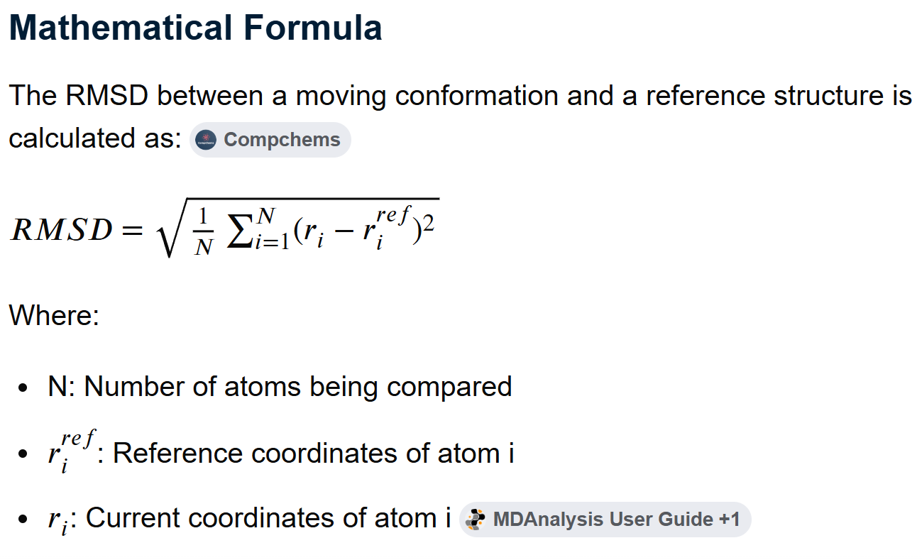
核心缺陷:它是全局平均统计量,丢失空间、局部、分布信息,只能输出一个单一数字。
RMSD是「退化指标 degenerate metric」
退化 = 多种完全不同的构象变化,能算出几乎一样的RMSD数值,一个RMSD值无法唯一对应一种构象变化模式,信息不可逆丢失。
举两组极端对比,最终RMSD完全相同,但稳定性天差地别:
场景A(看似高RMSD,但整体骨架极稳定)
超大蛋白复合物(几百个氨基酸),98%的主链原子几乎不动,只有一段柔性无序loop(20个残基)剧烈摆动,loop原子偏移1 nm。
大量不动原子稀释了局部大偏差,全局RMSD最终只算出来 0.1 nm,数值很小。
肉眼看:蛋白主体折叠完全不变,只有一段柔性尾巴晃。
场景B(低RMSD,但核心功能区已经变形)
小型球状蛋白,全部主链原子均匀轻微偏移0.09 nm,包括活性口袋、螺旋折叠核心。
全局RMSD同样 0.1 nm,和上面复合物数值一模一样。
肉眼看:蛋白核心折叠、功能位点整体变形,结构已经失稳。
关键矛盾:同一个RMSD数值,既可以代表「结构高度稳定仅柔性区波动」,也可以代表「全局骨架均匀变形、功能区破坏」。
仅看RMSD曲线平稳,你无法区分是哪种情况------这就是退化,单一数值丢失局部空间信息。
反向例子教程原文提到的:大型蛋白复合物RMSD达到1.0 nm,但结构很稳定。
原因:分子原子基数巨大,绝大多数原子固定,少数柔性区域的大幅偏移被海量静止原子平均稀释,全局RMSD数值被拉高,但核心折叠区域几乎无变化。你只看1.0 nm这个数字会误以为蛋白解折叠,实际完全相反。
RMSD是「外源性量 extrinsic quantity」
内源量 vs 外源量区分
- 内源指标 :只描述体系自身内部动力学、局部柔性,和分子尺寸、原子总数无关;代表:RMSF(残基波动)、回旋半径、二级结构占比、氢键数量。
不管蛋白大小,RMSF=0.2 Å都代表该残基柔性很高,有统一物理意义。 - 外源指标 :数值高度依赖体系原子总数、分子尺寸、计算组原子数量,不具备跨体系、跨蛋白对比的统一标准;RMSD就是典型外源量。
直观理解:
- 130个残基单域蛋白,平衡后主链RMSD稳定在0.09 nm;
- 1000残基多亚基复合物,哪怕结构几乎不变,主链RMSD天然容易达到0.4~1.0 nm;
两者数值差10倍,但不能说大复合物更不稳定------数值本身没有绝对评判标准。
你不能建立统一阈值:"RMSD<0.2 nm算稳定"。这条标准对小分子蛋白成立,对超大复合物完全失效。
因此无法靠RMSD数值大小定义"稳定/收敛",没有通用判定标尺。
RMSD只是微小偏差的全局累积,掩盖局部关键变化
RMSD是所有原子偏差的平方和平均,具备极强的"平均抹平效应":
- 少量关键残基的巨大构象改变,会被大量静止残基掩盖;
比如酶的活性中心5个残基完全解离、构象翻转,但其余300个主链原子纹丝不动,全局RMSD只上升0.05 nm,曲线看上去依旧平稳。
如果你只看RMSD,会完全错过活性位点失活这个核心结论。 - 全局轻微偏移累积,也会拉高RMSD,但不代表结构失稳;
整个蛋白均匀轻微舒展,无解折叠、无核心破坏,RMSD缓慢上升,属于正常水溶液弛豫,不是不稳定。
RMSD无法区分两种完全不同的变化:
① 局部关键结构剧烈扰动;② 全局均匀微小舒展。
收敛的定义本身,RMSD无法满足
模拟收敛的标准定义:体系所有可观测物理量的概率分布不再随模拟时间变化,需要证明:
- 各残基柔性分布稳定(RMSF曲线前后两段重合);
- 二级结构占比长期不变;
- 配体/蛋白氢键、盐桥、疏水相互作用数量稳定;
- 自由能、回旋半径等热力学参数分布收敛;
而RMSD只是单一全局平均值,哪怕RMSD曲线后期走平,也只能说明"整体平均偏移不再增加",不能证明:
- 局部柔性区域的波动分布收敛;
- 蛋白二级结构没有持续丢失;
- 结合口袋构象在持续重构。
举个反例:
模拟前5 ns RMSD快速上升,5--10 ns曲线完全平稳;但RMSF显示后半段loop残基波动范围持续变大,α螺旋占比线性下降。
此时RMSD看似收敛,但结构实际在持续失稳,仅靠RMSD会得出完全错误的结论。
RMSD的正确定位(不是不能用,是不能单独用来判定收敛/稳定)
- RMSD的合理用途
- 定性观察:模拟前期体系弛豫快慢,判断多久后整体构象不再大幅偏离初始态;
- 辅助对照:同一套体系下,对比有无配体、不同突变体之间整体偏移差异;
- 筛时间区间:粗略剔除前期剧烈弛豫阶段,缩小后续分析窗口。
- 绝对禁止单独依靠RMSD下结论
因为:
① 退化指标:多种构象变化对应同一RMSD,丢失局部信息;
② 外源量:数值依赖蛋白尺寸,无通用稳定阈值;
③ 平均抹平效应:掩盖活性中心、功能区域的关键局部变形;
④ 不满足收敛判定标准,单一全局值无法代表全体系热力学分布稳定。 - 完整、严谨的稳定性/收敛判定组合(论文通用)
RMSD(全局趋势) + RMSF(残基局部柔性) + 二级结构时序 + 回旋半径 + 关键相互作用(氢键/盐桥)。
Analyzing Compactness: Rg 分析紧密度:选转半径
Rg这个概念我们提过,就是分子动所有原子到其质心的均方根距离(距离平方,均值,再开根号)
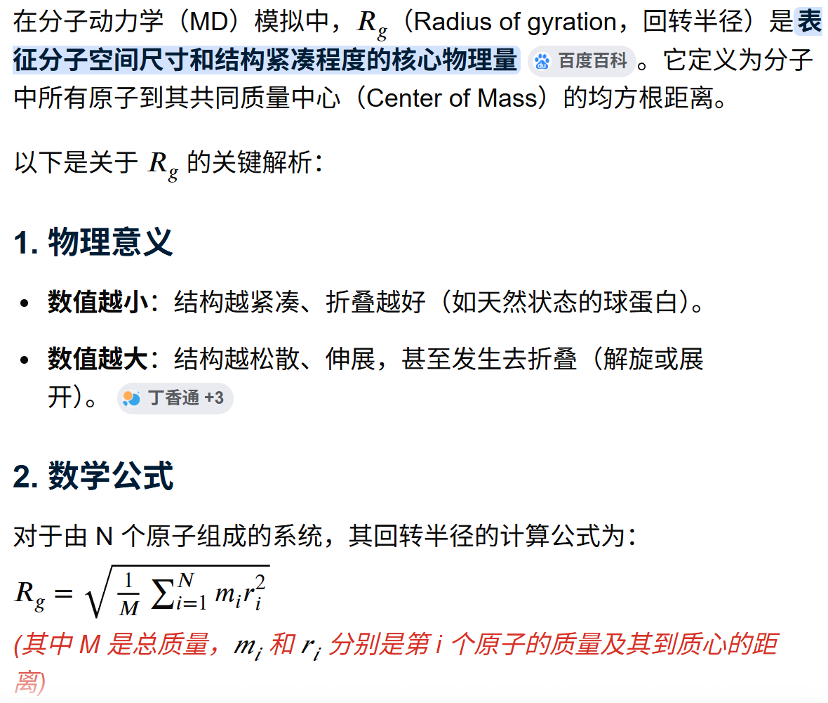
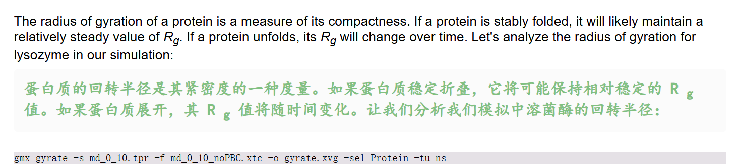
因为下面要用到gmx gyrate命令,同样
这个命令本质是,计算时间分辨回转半径 Rg + 三轴分量 Rx/Ry/Rz,定量判断生物大分子(蛋白 / DNA / 复合物)折叠、舒展、压缩、解折叠行为
python
gmx gyrate
gmx help gyrate
命令行输出日志如下,
python
Executable:   /home/csn/program/miniconda3/envs/gromacs/bin.AVX2_256/gmx
Data prefix:  /home/csn/program/miniconda3/envs/gromacs
Working dir:  /mnt/sdb/zht/project/tf-dna-md/files/structure/test
Command line:
  gmx help gyrate

SYNOPSIS

gmx gyrate [-f [<.xtc/.trr/...>]] [-s [<.tpr/.gro/...>]] [-n [<.ndx>]]
           [-o [<.xvg>]] [-b <time>] [-e <time>] [-dt <time>] [-tu <enum>]
           [-fgroup <selection>] [-xvg <enum>] [-[no]rmpbc] [-sf <file>]
           [-selrpos <enum>] [-seltype <enum>] [-sel <selection>]
           [-mode <enum>]

DESCRIPTION

gmx gyrate computes the radius of gyration of a molecule and the radii of
gyration about the x-, y- and z-axes, as a function of time. The atoms are
explicitly mass weighted.

The axis components corresponds to the mass-weighted root-mean-square of the
radii components orthogonal to each axis, for example:

Rg(x) = sqrt((sum_i w_i (R_i(y)^2 + R_i(z)^2))/(sum_i w_i)).

where w_i is the weight value in the given situation (mass, charge, unit)

Note that this is a new implementation of the gyrate utility added in GROMACS
2024. If you need the old one, use gmx gyrate-legacy.

OPTIONS

Options to specify input files:

 -f      [<.xtc/.trr/...>]  (traj.xtc)       (Opt.)
           Input trajectory or single configuration: xtc trr cpt gro g96 pdb
           tng
 -s      [<.tpr/.gro/...>]  (topol.tpr)      (Opt.)
           Input structure: tpr gro g96 pdb brk ent
 -n      [<.ndx>]           (index.ndx)      (Opt.)
           Extra index groups

Options to specify output files:

 -o      [<.xvg>]           (gyrate-taf.xvg)
           Filename for gyrate plot output

Other options:

 -b      <time>             (0)
           First frame (ps) to read from trajectory
 -e      <time>             (0)
           Last frame (ps) to read from trajectory
 -dt     <time>             (0)
           Only use frame if t MOD dt == first time (ps)
 -tu     <enum>             (ps)
           Unit for time values: fs, ps, ns, us, ms, s
 -fgroup <selection>
           Atoms stored in the trajectory file (if not set, assume first N
           atoms)
 -xvg    <enum>             (xmgrace)
           Plot formatting: xmgrace, xmgr, none
 -[no]rmpbc                 (yes)
           Make molecules whole for each frame
 -sf     <file>
           Provide selections from files
 -selrpos <enum>            (atom)
           Selection reference positions: atom, res_com, res_cog, mol_com,
           mol_cog, whole_res_com, whole_res_cog, whole_mol_com,
           whole_mol_cog, part_res_com, part_res_cog, part_mol_com,
           part_mol_cog, dyn_res_com, dyn_res_cog, dyn_mol_com, dyn_mol_cog
 -seltype <enum>            (atom)
           Default selection output positions: atom, res_com, res_cog,
           mol_com, mol_cog, whole_res_com, whole_res_cog, whole_mol_com,
           whole_mol_cog, part_res_com, part_res_cog, part_mol_com,
           part_mol_cog, dyn_res_com, dyn_res_cog, dyn_mol_com, dyn_mol_cog
 -sel    <selection>
           Select group to compute gyrate radius
 -mode   <enum>             (mass)
           Atom weighting mode: mass, charge, geometry

GROMACS reminds you: "It's Against the Rules" (Pulp Fiction)
整体上gyrate的语法如下
python
gmx gyrate [-f 轨迹] [-s 拓扑] [-n 索引组]
           [-o 输出曲线] [-b/-e/-dt 帧控制] [-tu 时间单位]
           [-fgroup] [-xvg 绘图格式] [-[no]rmpbc] [-sf 选择文件]
           [-selrpos/-seltype/-sel 原子选择] [-mode 权重模式]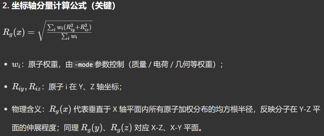
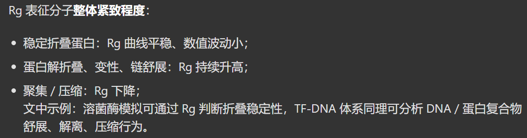
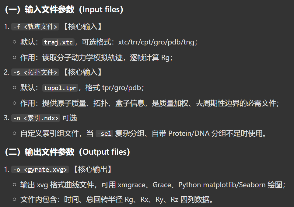
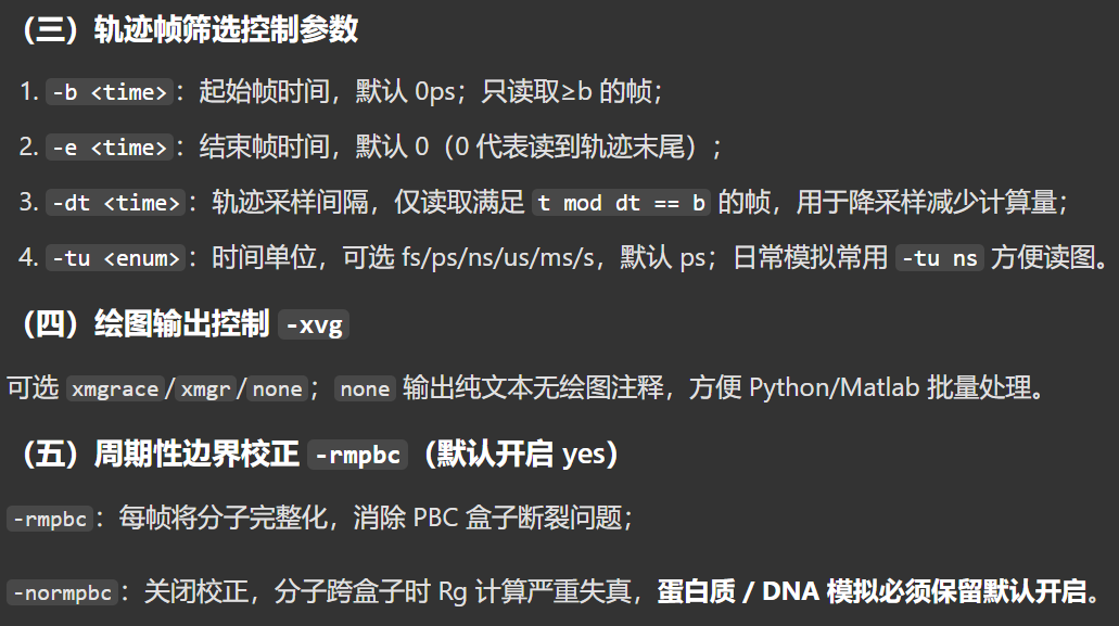
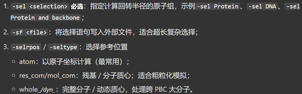
然后下面是我们要运行的命令
python
gmx gyrate -s md_0_10.tpr -f md_0_10_noPBC.xtc -o gyrate.xvg -sel Protein -tu ns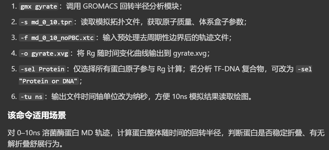
python
Command line:
  gmx gyrate -s md_0_10.tpr -f md_0_10_noPBC.xtc -o gyrate.xvg -sel Protein -tu ns

Reading file md_0_10.tpr, VERSION 2025.4-conda_forge (single precision)
Reading file md_0_10.tpr, VERSION 2025.4-conda_forge (single precision)
# 一共完整读取、计算了 1001 帧(0~1000 帧首尾都包含)
# 整条 10 ns 轨迹全部完成回转半径计算,无截断、无报错,gyrate.xvg 包含全部 1001 个时间点的 Rg、Rx/Ry/Rz 数据
Last frame       1000 time   10.000
Analyzed 1001 frames, last time 10000.000

GROMACS reminds you: "If all it takes to motivate you is a fancy picture and quote, you probably have a very easy job. The type of job computers will soon be doing." (Anonymous)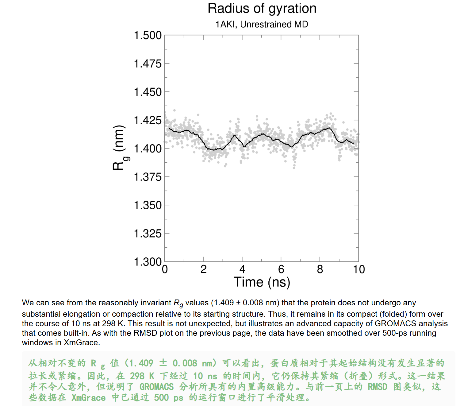
同样的使用我们前面开发的工具自己来可视化一下:
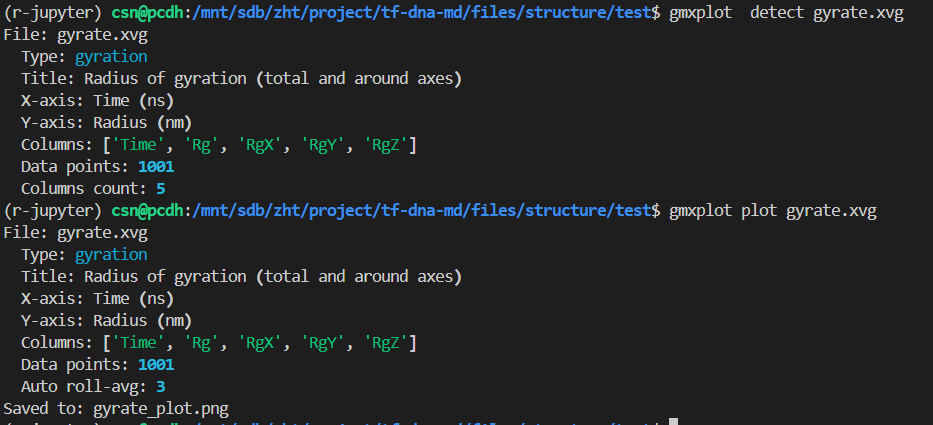
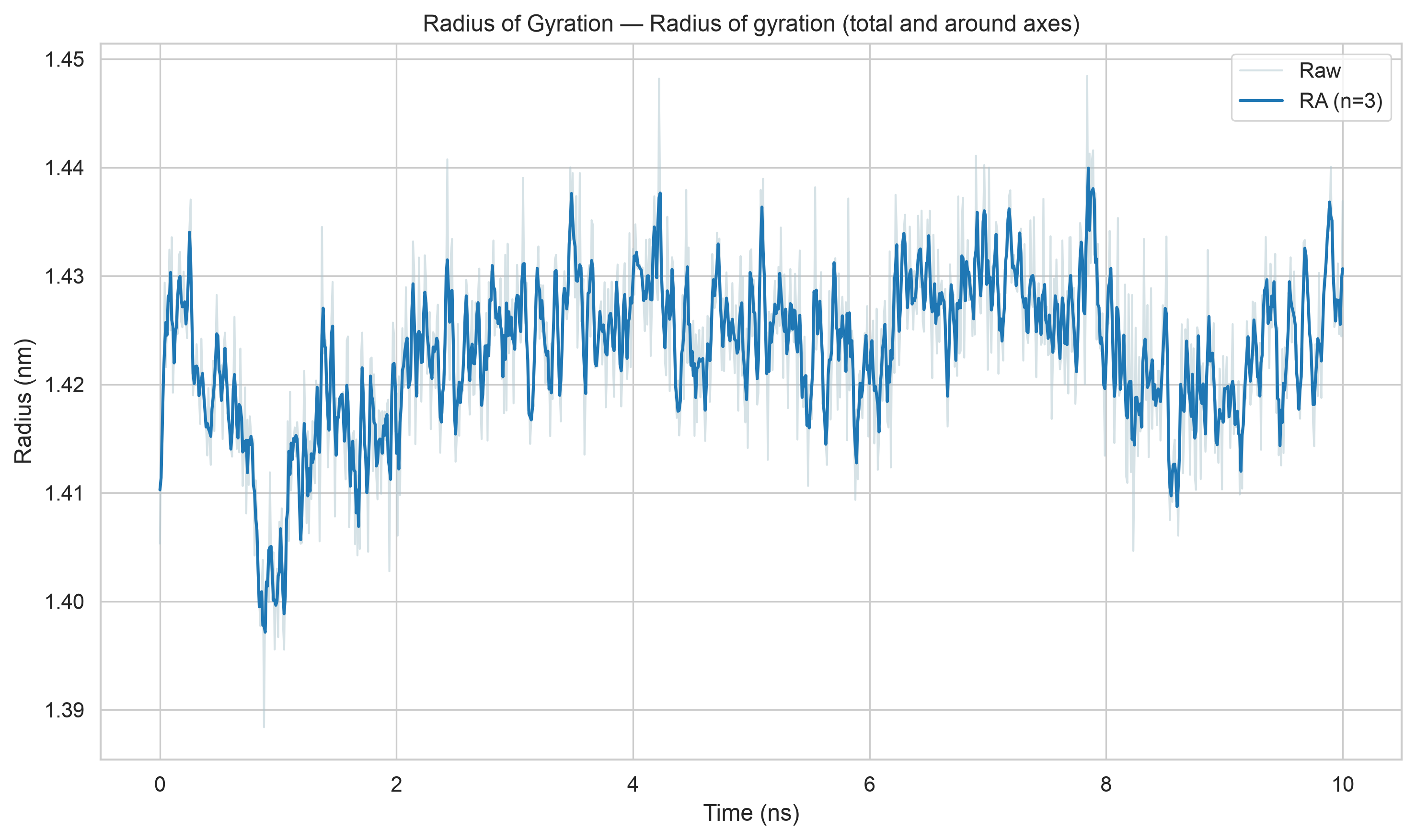
再次注意,我们这里的滑动窗口平均和xmgrace处理的不一致(按照教程是500ps窗口滑动平均)。
Secondary Structure 二级结构
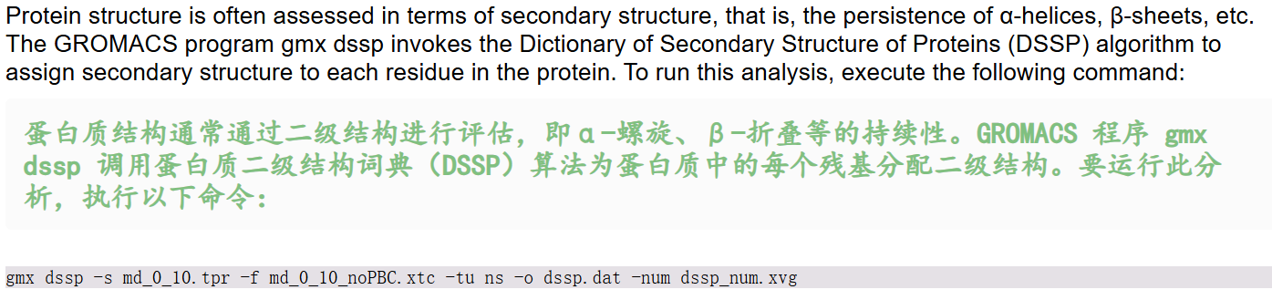
因为需要用到gmx dssp命令,所以我们同样先查看一下文档:
这个命令基于DSSP 标准算法,通过残基间氢键模式识别,逐残基判定蛋白质二级结构,逐帧追踪模拟过程中二级结构随时间的变化;
python
gmx dssp
gmx help dssp
# gmx dssp -h
python
Executable:   /home/csn/program/miniconda3/envs/gromacs/bin.AVX2_256/gmx
Data prefix:  /home/csn/program/miniconda3/envs/gromacs
Working dir:  /mnt/sdb/zht/project/tf-dna-md/files/structure/test
Command line:
  gmx dssp -h

SYNOPSIS

gmx dssp [-f [<.xtc/.trr/...>]] [-s [<.tpr/.gro/...>]] [-n [<.ndx>]]
         [-o [<.dat>]] [-num [<.xvg>]] [-b <time>] [-e <time>] [-dt <time>]
         [-tu <enum>] [-fgroup <selection>] [-xvg <enum>] [-[no]rmpbc]
         [-[no]pbc] [-sf <file>] [-selrpos <enum>] [-seltype <enum>]
         [-sel <selection>] [-hmode <enum>] [-hbond <enum>] [-[no]nb]
         [-cutoff <real>] [-[no]clear] [-[no]pihelix] [-ppstretch <enum>]
         [-[no]polypro]

DESCRIPTION

gmx dssp allows using the DSSP algorithm (namely, by detecting specific
patterns of hydrogen bonds between amino acid residues) to determine the
secondary structure of a protein.

One-symbol secondary structure designations that are used in the output file:

H --- alpha-helix;

B --- residue in isolated beta-bridge;

E --- extended strand that participates in beta-ladder;

G --- 3_10-helix;

I --- pi-helix;

P --- kappa-helix (poly-proline II helix);

S --- bend;

T --- hydrogen-bonded turn;

= --- break;

~ --- loop (no special secondary structure designation).

-num allows you to get a plot of the number of secondary structures of each
type as a function of time at the output.

-hmode selects between using hydrogen atoms directly from the structure
("gromacs" option) and using hydrogen pseudo-atoms based on C and O atom
coordinates of previous residue ("dssp" option). You should always use the
"dssp" option for structures with absent hydrogen atoms!

-hbond selects between different definitions of hydrogen bond. "energy" means
the calculation of a hydrogen bond using the electrostatic interaction energy
and "geometry" means the calculation of the hydrogen bond using geometric
criterion for the existence of a hydrogen bond.

-nb allows using GROMACS neighbor-search method to find residue pairs that may
have a hydrogen bond instead of simply iterating over the residues among
themselves.

-cutoff is a real value that defines maximum distance from residue to its
neighbor residue used in -nb. Minimum (and also recommended) value is 0.9.

-clear allows you to ignore the analysis of the secondary structure residues
that are missing one or more critical atoms (CA, C, N, O or H). Always use
this option together with -hmode dssp for structures that lack hydrogen atoms!

-pihelix changes pattern-search algorithm towards preference of pi-helices.

-ppstretch defines stretch value of polyproline-helices. "shortened" means
stretch with size 2 and "default" means stretch with size 3.

-polypro enables the search for polyproline helices (default behavior,
equivalent to DSSP v4). Disabling this option will result in disabling the
search for polyproline helices, reproducing the behavior of DSSP v2.

Note that gmx dssp currently is not capable of reproducing the secondary
structure of proteins whose structure is determined by methods other than
X-ray crystallography (structures in .pdb format with incorrect values in the
CRYST1 line) due to the incorrect cell size in such structures.

Please note that the computation is always done in single precision,
regardless of the precision for which GROMACS was configured.

OPTIONS

Options to specify input files:

 -f      [<.xtc/.trr/...>]  (traj.xtc)       (Opt.)
           Input trajectory or single configuration: xtc trr cpt gro g96 pdb
           tng
 -s      [<.tpr/.gro/...>]  (topol.tpr)      (Opt.)
           Input structure: tpr gro g96 pdb brk ent
 -n      [<.ndx>]           (index.ndx)      (Opt.)
           Extra index groups

Options to specify output files:

 -o      [<.dat>]           (dssp.dat)
           Filename for DSSP output
 -num    [<.xvg>]           (num.xvg)        (Opt.)
           Output file name for secondary structures statistics for the
           trajectory

Other options:

 -b      <time>             (0)
           First frame (ps) to read from trajectory
 -e      <time>             (0)
           Last frame (ps) to read from trajectory
 -dt     <time>             (0)
           Only use frame if t MOD dt == first time (ps)
 -tu     <enum>             (ps)
           Unit for time values: fs, ps, ns, us, ms, s
 -fgroup <selection>
           Atoms stored in the trajectory file (if not set, assume first N
           atoms)
 -xvg    <enum>             (xmgrace)
           Plot formatting: xmgrace, xmgr, none
 -[no]rmpbc                 (yes)
           Make molecules whole for each frame
 -[no]pbc                   (yes)
           Use periodic boundary conditions for distance calculation
 -sf     <file>
           Provide selections from files
 -selrpos <enum>            (atom)
           Selection reference positions: atom, res_com, res_cog, mol_com,
           mol_cog, whole_res_com, whole_res_cog, whole_mol_com,
           whole_mol_cog, part_res_com, part_res_cog, part_mol_com,
           part_mol_cog, dyn_res_com, dyn_res_cog, dyn_mol_com, dyn_mol_cog
 -seltype <enum>            (atom)
           Default selection output positions: atom, res_com, res_cog,
           mol_com, mol_cog, whole_res_com, whole_res_cog, whole_mol_com,
           whole_mol_cog, part_res_com, part_res_cog, part_mol_com,
           part_mol_cog, dyn_res_com, dyn_res_cog, dyn_mol_com, dyn_mol_cog
 -sel    <selection>
           Group for DSSP
 -hmode  <enum>             (gromacs)
           Hydrogens pseudoatoms creating mode: gromacs, dssp
 -hbond  <enum>             (energy)
           Selects between different definitions of hydrogen bond: energy,
           geometry
 -[no]nb                    (yes)
           Use GROMACS neighbor-search method
 -cutoff <real>             (0.9)
           Distance from residue to its neighbor residue in neighbor search.
           Must be >= 0.9
 -[no]clear                 (no)
           Clear defective residues from the structure
 -[no]pihelix               (no)
           Prefer Pi Helices
 -ppstretch <enum>          (default)
           Stretch value for PP-helices: shortened, default
 -[no]polypro               (yes)
           Perform a search for polyproline helices

GROMACS reminds you: "It Doesn't Seem Right, No Computers in Sight" (Faun Fables)
对于二级结构编码:
| 符号 | 结构类型 |
|---|---|
| H | α 螺旋 |
| B | 孤立 β 桥残基 |
| E | 参与 β 折叠链 |
| G | 3₁₀螺旋 |
| I | π 螺旋 |
| P | 聚脯氨酸 II 螺旋 |
| S | 弯曲 |
| T | 氢键转角 |
| = | 结构断裂 |
| ~ | 无规卷曲 / 环区 |
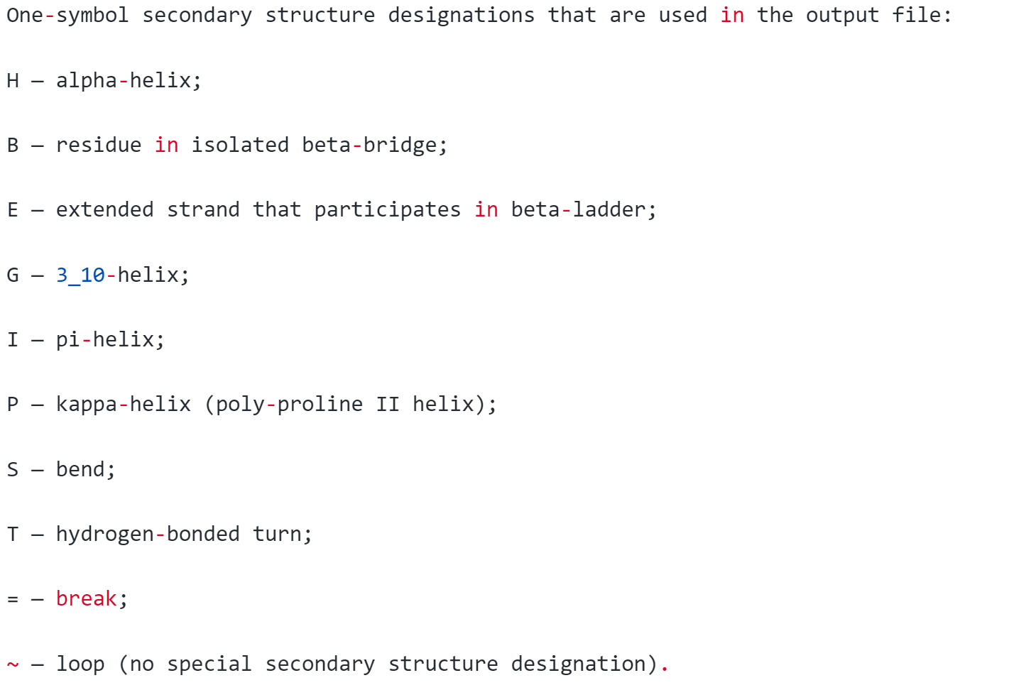
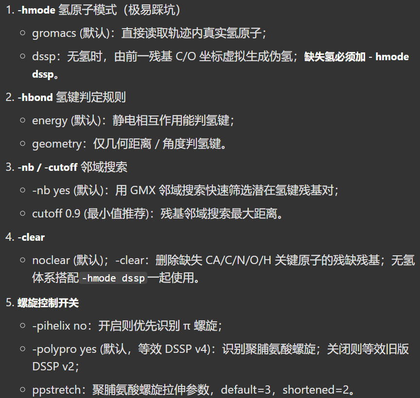
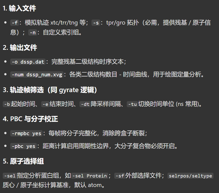
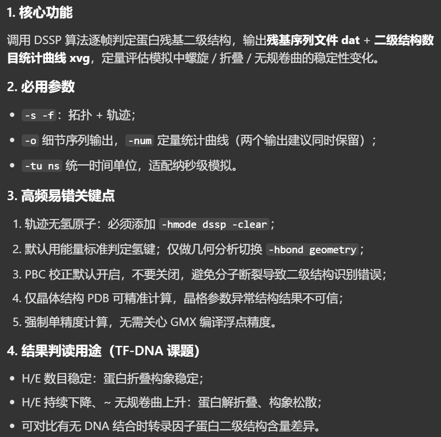
比如说这里可以选择有无某一段结构域时,TF-DNA的二级结构的一个含量比例的相对变化
我们的命令如下
python
gmx dssp -s md_0_10.tpr -f md_0_10_noPBC.xtc -tu ns -o dssp.dat -num dssp_num.xvg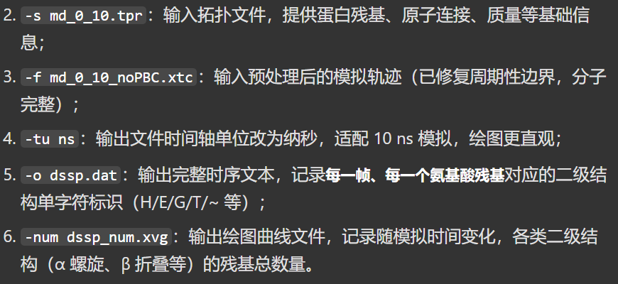
输出运行日志如下
python
Command line:
  gmx dssp -s md_0_10.tpr -f md_0_10_noPBC.xtc -tu ns -o dssp.dat -num dssp_num.xvg

Reading file md_0_10.tpr, VERSION 2025.4-conda_forge (single precision)
Reading file md_0_10.tpr, VERSION 2025.4-conda_forge (single precision)
# 完整计算全部 0~1000 共 1001 帧;内部原始时间单位 ps,10000 ps = 10 ns,轨迹全部分析完成,无报错
Last frame       1000 time   10.000
Analyzed 1001 frames, last time 10000.000

++++ PLEASE READ AND CITE THE FOLLOWING REFERENCE ++++
W. Kabsch, C. Sander
Dictionary of protein secondary structure: pattern recognition of
hydrogen-bonded and geometrical features
Biopolymers (1983)
DOI: 10.1002/bip.360221211
-------- -------- --- Thank You --- -------- --------


++++ PLEASE READ AND CITE THE FOLLOWING REFERENCE ++++
S. Gorelov, A. Titov, O. Tolicheva, A. Konevega, A. Shvetsov
DSSP in GROMACS: Tool for Defining Secondary Structures of Proteins in
Trajectories
Journal of Chemical Information and Modeling (2024)
DOI: 10.1021/acs.jcim.3c01344
-------- -------- --- Thank You --- -------- --------
输出两个文件
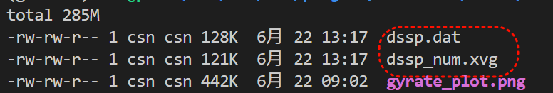
首先是这个dat文本文件,总共1001帧,每一帧的二级机构统计量
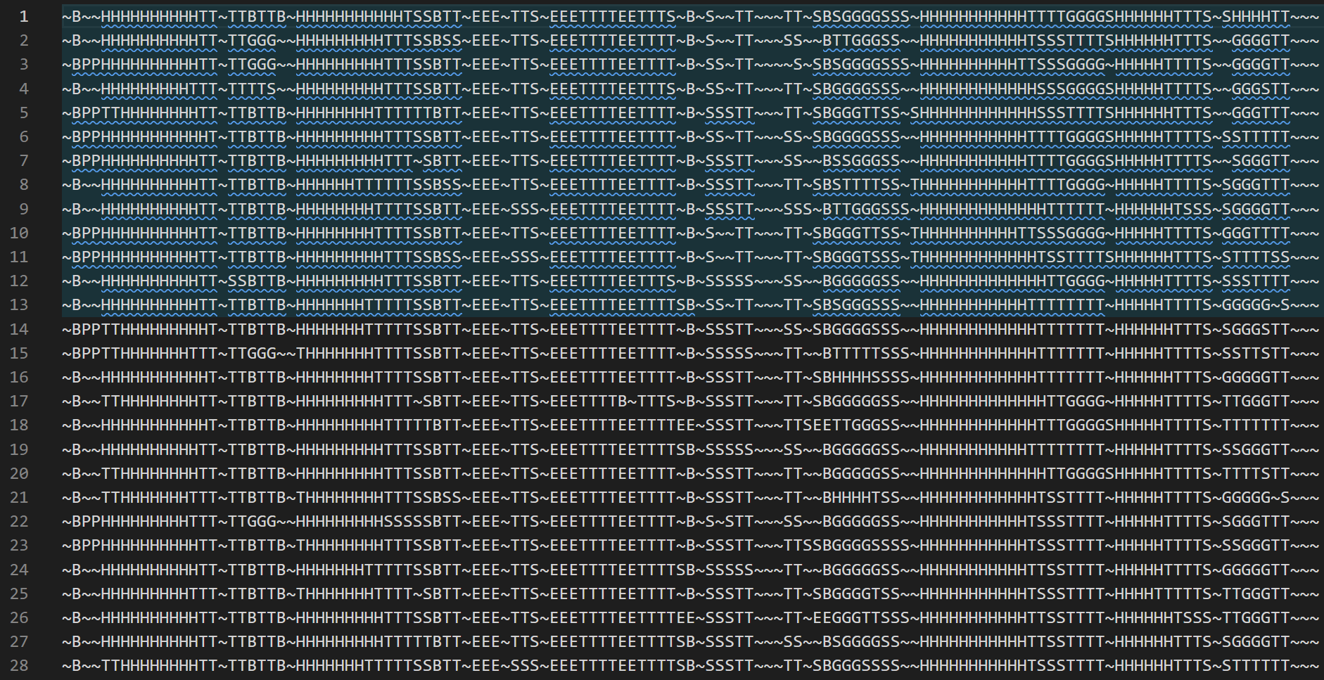

至于dssp的xvg文件
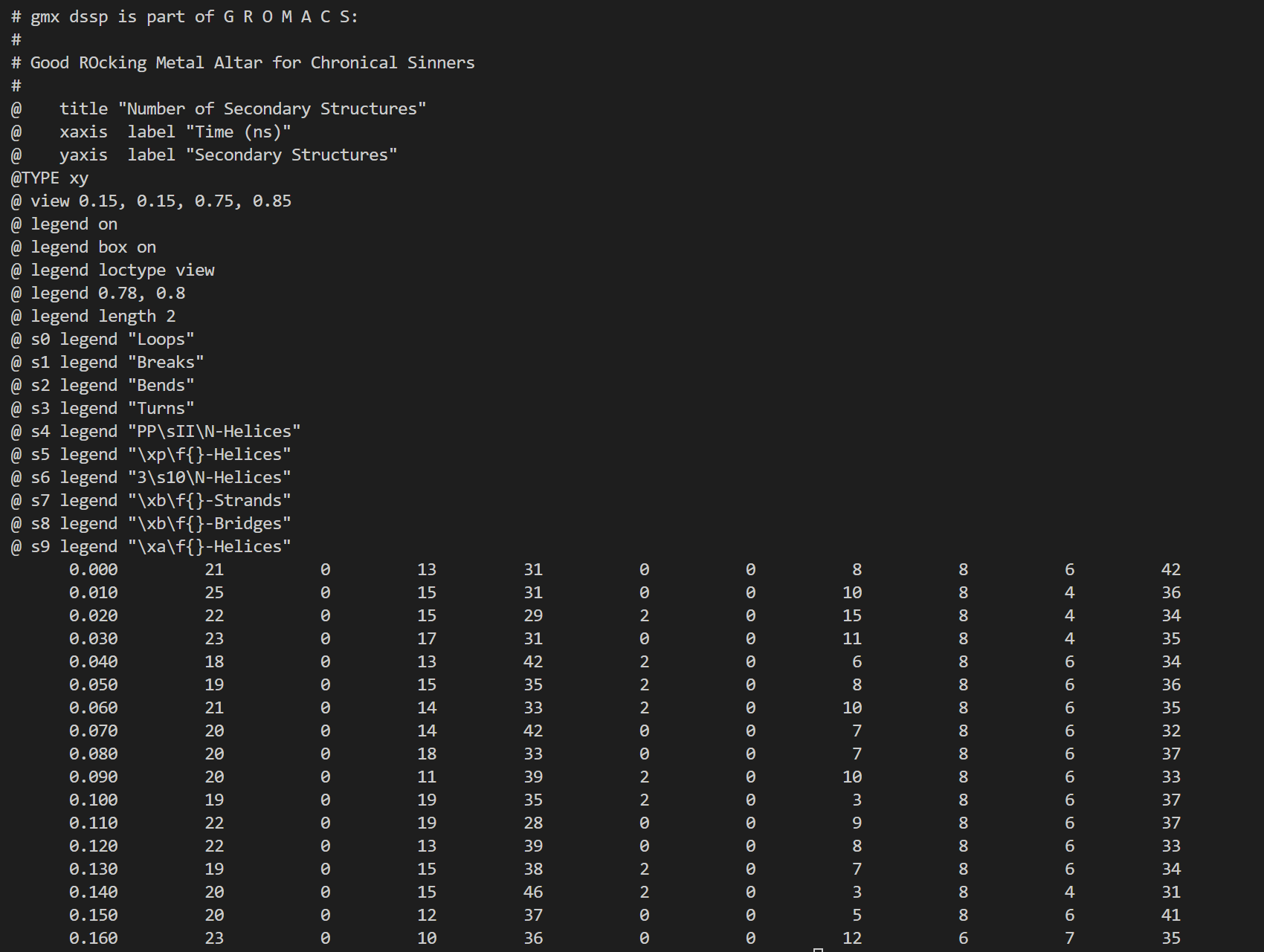
同样用我们前面的工具
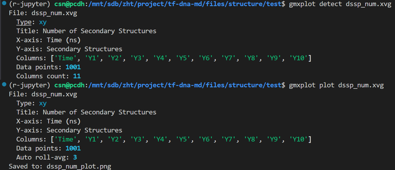
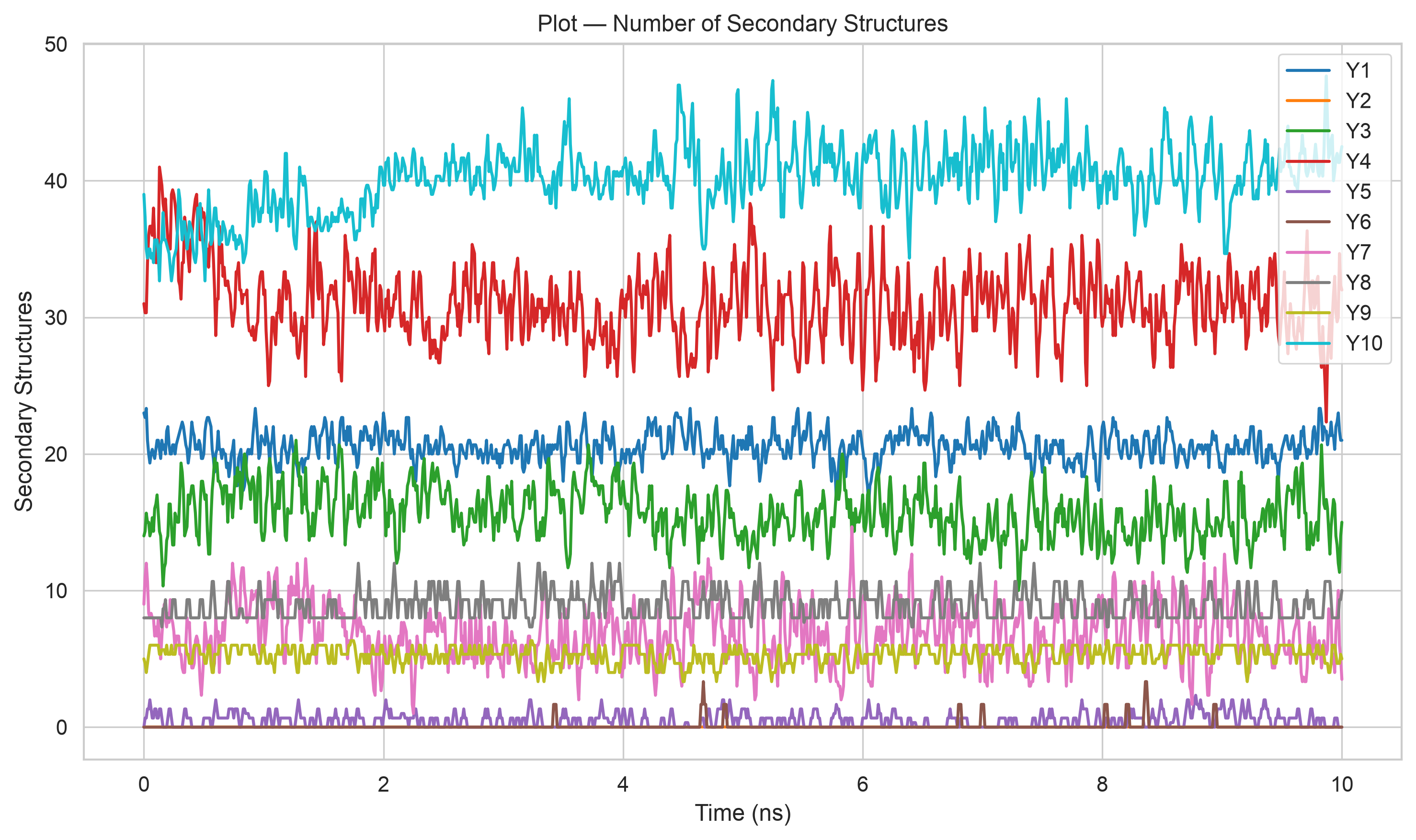
可以看到,基本上还是没怎么变化
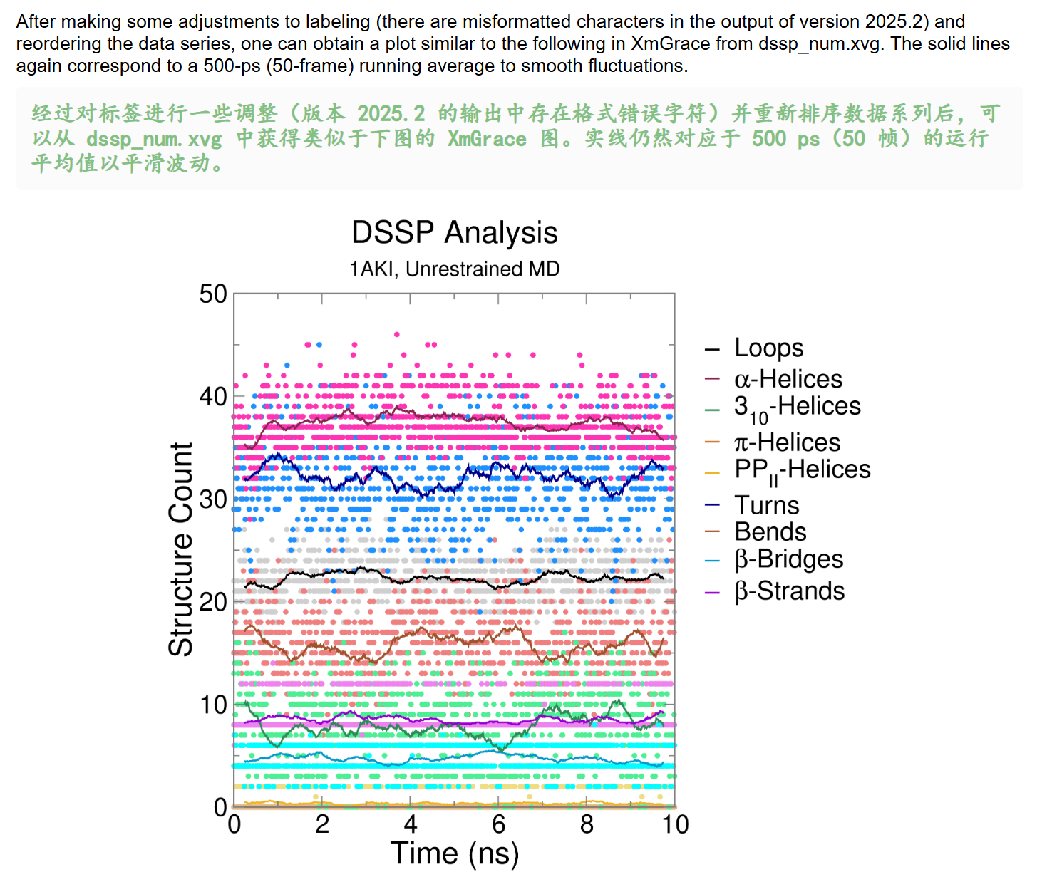
Hydrogen Bonds 氢键
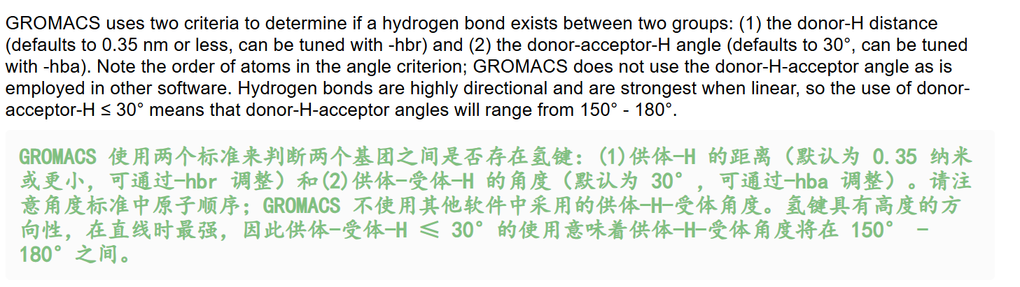
⚠️ 注意!这个教程中的定义有问题,我们需要搞清楚氢键一般的定义
什么是氢键?
我们先来解释一下什么是氢键:
参考:https://zh.wikipedia.org/wiki/氢键
简单来说就是通过共价键和某一个原子X相连的H原子和另外一个原子Y之间形成的相互作用,
然后这两个原子X、Y都是电负性比较强的
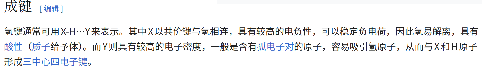
- X-H ... Y
- X以共价键与氢相连,电负性较高,可以稳定负电荷,然后氢容易解离,具有酸性,质子给体
- Y具有较高的电子密度,一般是含有孤电子对的原子,容易吸引氢原子,质子受体
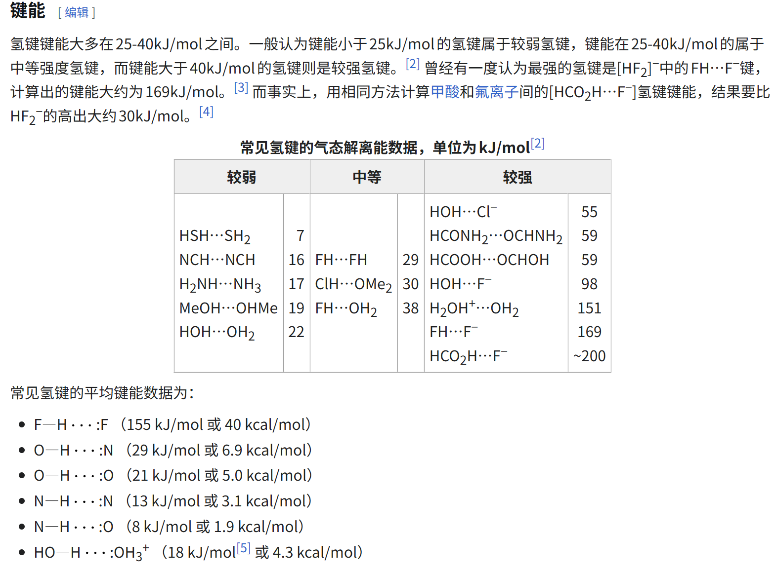
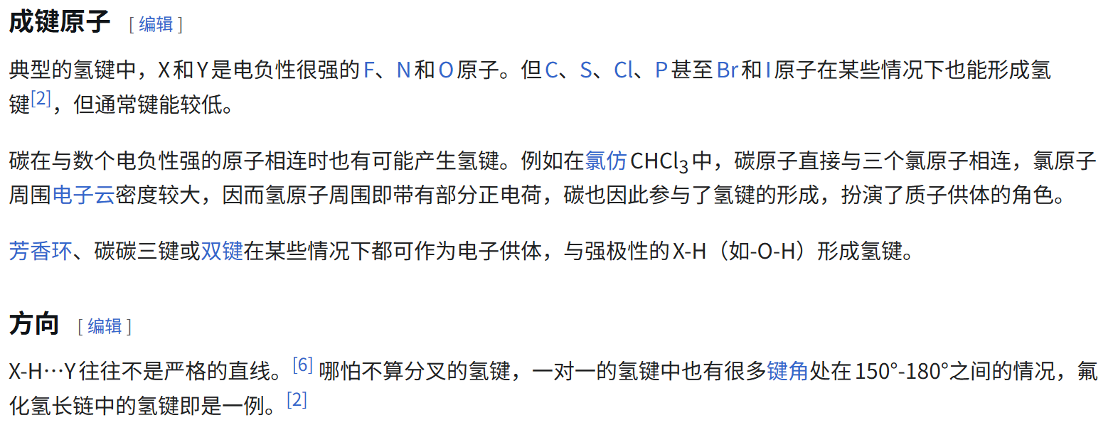
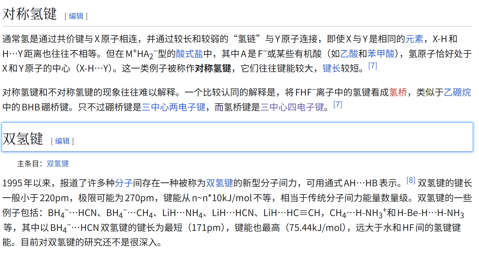
比较重要的其实就是分子间氢键,以及分子内氢键
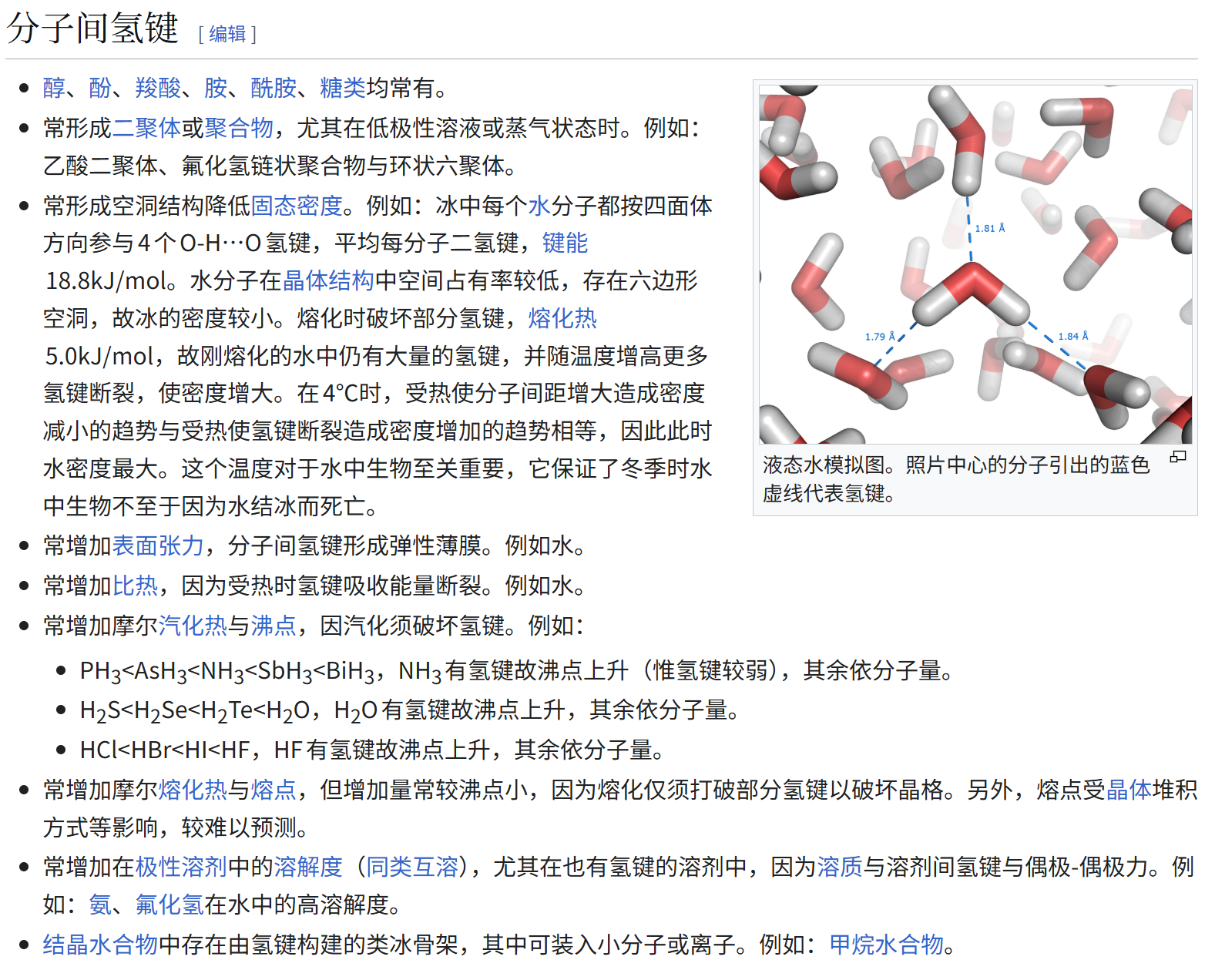
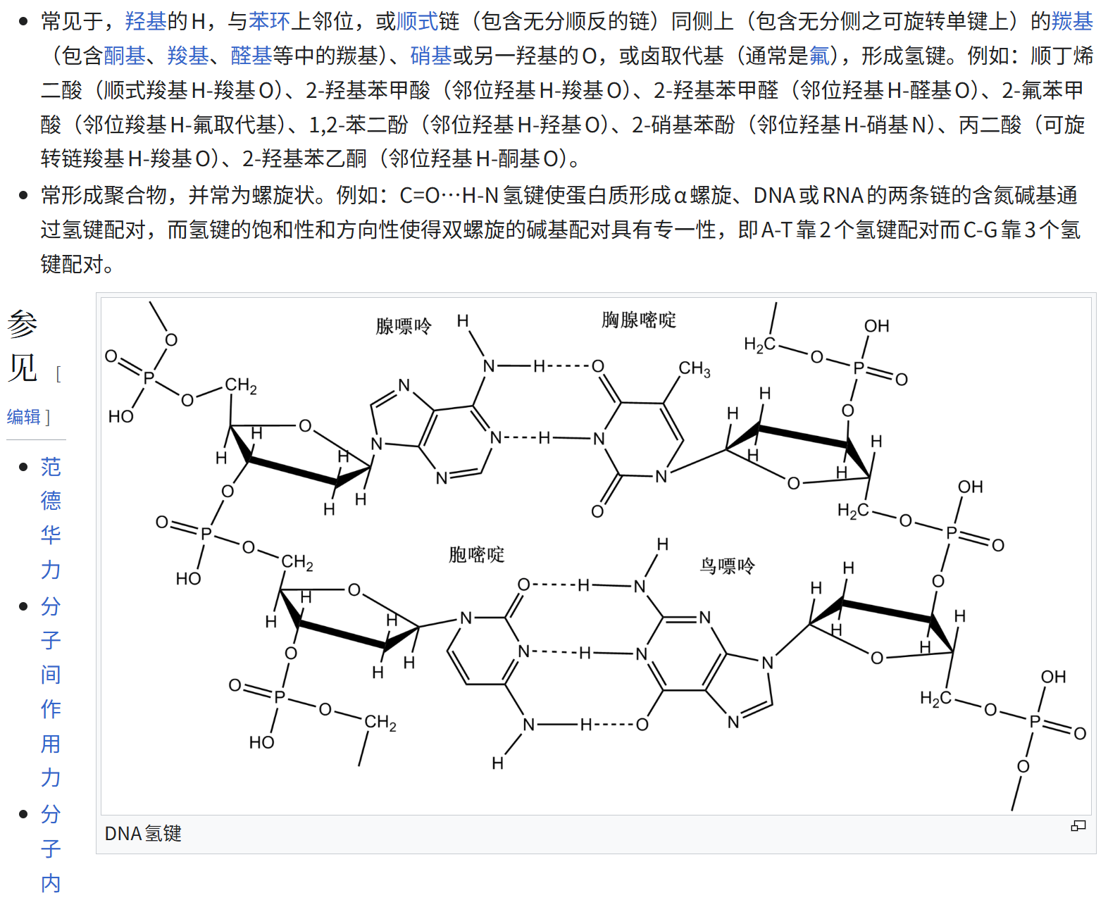
回到gromacs
现在回到我们前面的教程:
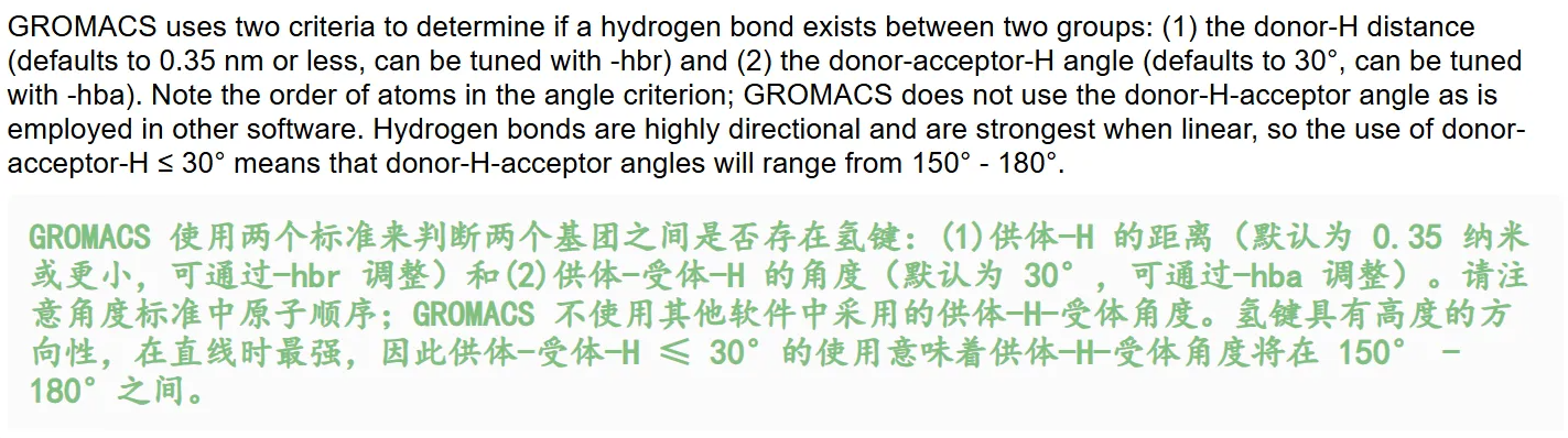
对于氢键的判断标准:
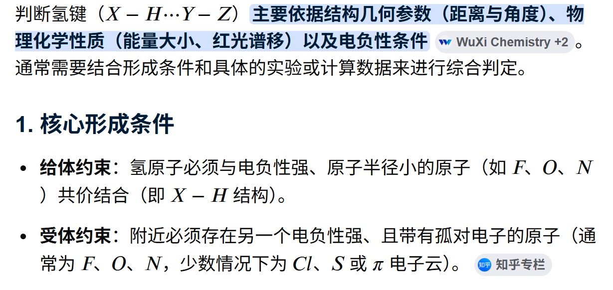
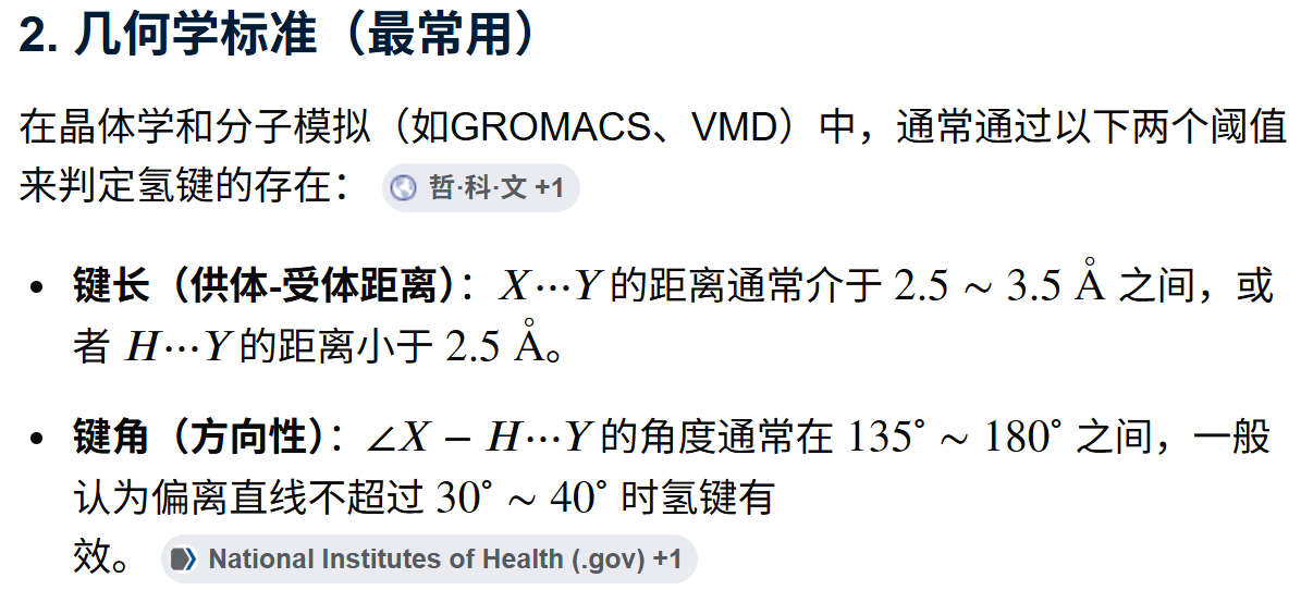
可以看到,在判断标准上,gromacs没有从定义、键能出发,而是采用了最简单直接的几何学标准,
涉及到判断的两个方面是没有问题的:
- 距离
- 角度
但是这个数据上有问题,就像我们前面说的那样,这毕竟是1个第三方教程,虽然在官方推荐列表中,但是有错误还是难免的。
我们参考官方说明:https://manual.gromacs.org/current/reference-manual/analysis/hydrogen-bonds.html
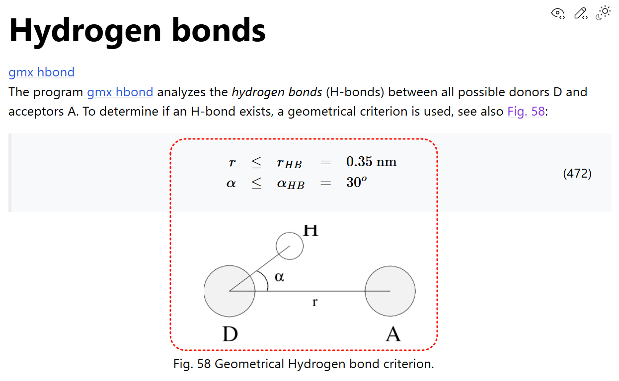
gromacs对于氢键的判断标准:
- 供体-受体 距离(一般是≤0.35nm)
- H-供体-受体 角度(一般是≤30°)
因为接下来会用到gmx hbond命令,所以同样:
这个命令简单来说,就是基于几何判据统计两组原子间 / 组内所有氢键,输出氢键数量时序、距离 / 角度分布、供受体统计、氢键原子索引文件
python
gmx hbond
gmx help hbond
输出指示文档如下
python
Executable:   /home/csn/program/miniconda3/envs/gromacs/bin.AVX2_256/gmx
Data prefix:  /home/csn/program/miniconda3/envs/gromacs
Working dir:  /mnt/sdb/zht/project/tf-dna-md/files/structure/test
Command line:
  gmx help hbond

SYNOPSIS

gmx hbond [-f [<.xtc/.trr/...>]] [-s [<.tpr/.gro/...>]] [-n [<.ndx>]]
          [-o [<.ndx>]] [-num [<.xvg>]] [-dist [<.xvg>]] [-ang [<.xvg>]]
          [-dan [<.xvg>]] [-b <time>] [-e <time>] [-dt <time>] [-tu <enum>]
          [-fgroup <selection>] [-xvg <enum>] [-[no]rmpbc] [-[no]pbc]
          [-sf <file>] [-selrpos <enum>] [-seltype <enum>] [-r <selection>]
          [-t <selection>] [-[no]m] [-[no]pf] [-cutoff <real>] [-hbr <real>]
          [-hba <real>] [-de <string>] [-ae <string>]

DESCRIPTION

gmx hbond allows using geometric definition of hydrogen bonds to define them
throughout the structure.

-r specifies reference selection, relative to which the search for hydrogen
bonds in target selection will develop. Note that all atoms in reference and
target selections should be either absolutely identical or non-overlapping at
all. Accepts dynamic selection.

-t specifies target selection, relative to which the search for hydrogen bonds
in reference selection will develop. Note that all atoms in reference and
target selections should be either absolutely identical or non-overlapping at
all. Accepts dynamic selection.

-m forces to merge together information in output index file about hydrogen
bonds if they differ only in hydrogen indices. This also means that
information about hydrogen atoms in the hydrogen bonds would not be written in
output index file at all.

-pf forces to write hydrogen bonds for each frame separately instead of
writing hydrogen bonds for the whole system. Each information about hydrogen
bonds in new frame will be stored in its own section of the output index file.

-cutoff is a real value that defines distance from donor to acceptor (and vice
versa) that used in neighbor search. Minimum (and also recommended) value is
0.35.

-hbr Sets the cutoff that is used when calculating hydrogen bond distances.
Recommended value: 0.35.

-hba Sets the cutoff that is used when calculating hydrogen bond angles.
Recommended value: 30.

-de Specifies the atomic elements that will be selected from the topology to
check if a given element is a potential hydrogen bond donor.

-ae Specifies the atomic elements that will be selected from the topology to
check if a given element is a potential hydrogen bond acceptor.

-num allows you to get a plot of the number of hydrogen bonds as a function of
time at the output.

-dist allows you to get a plot of the distance distribution of all hydrogen
bonds at the output.

-ang allows you to get a plot of the angular distribution of all hydrogen
bonds at the output.

-dan allows you to get a plot of the number of analyzed donors and acceptors
for each frame at the output.

Note that this is a new implementation of the hbond utility added in GROMACS
2024. If you need the old one, use gmx hbond-legacy.

OPTIONS

Options to specify input files:

 -f      [<.xtc/.trr/...>]  (traj.xtc)       (Opt.)
           Input trajectory or single configuration: xtc trr cpt gro g96 pdb
           tng
 -s      [<.tpr/.gro/...>]  (topol.tpr)      (Opt.)
           Input structure: tpr gro g96 pdb brk ent
 -n      [<.ndx>]           (index.ndx)      (Opt.)
           Extra index groups

Options to specify output files:

 -o      [<.ndx>]           (hbond.ndx)
           Index file that contains selected groups', acceptors', donors' and
           hydrogens' indices and hydrogen bond pairs between or within
           selected groups.
 -num    [<.xvg>]           (hbnum.xvg)      (Opt.)
           Number of hydrogen bonds as a function of time.
 -dist   [<.xvg>]           (hbdist.xvg)     (Opt.)
           Distance distribution of all hydrogen bonds.
 -ang    [<.xvg>]           (hbang.xvg)      (Opt.)
           Angle distribution of all hydrogen bonds.
 -dan    [<.xvg>]           (hbdan.xvg)      (Opt.)
           Number of donors and acceptors analyzed for each frame.

Other options:

 -b      <time>             (0)
           First frame (ps) to read from trajectory
 -e      <time>             (0)
           Last frame (ps) to read from trajectory
 -dt     <time>             (0)
           Only use frame if t MOD dt == first time (ps)
 -tu     <enum>             (ps)
           Unit for time values: fs, ps, ns, us, ms, s
 -fgroup <selection>
           Atoms stored in the trajectory file (if not set, assume first N
           atoms)
 -xvg    <enum>             (xmgrace)
           Plot formatting: xmgrace, xmgr, none
 -[no]rmpbc                 (yes)
           Make molecules whole for each frame
 -[no]pbc                   (yes)
           Use periodic boundary conditions for distance calculation
 -sf     <file>
           Provide selections from files
 -selrpos <enum>            (atom)
           Selection reference positions: atom, res_com, res_cog, mol_com,
           mol_cog, whole_res_com, whole_res_cog, whole_mol_com,
           whole_mol_cog, part_res_com, part_res_cog, part_mol_com,
           part_mol_cog, dyn_res_com, dyn_res_cog, dyn_mol_com, dyn_mol_cog
 -seltype <enum>            (atom)
           Default selection output positions: atom, res_com, res_cog,
           mol_com, mol_cog, whole_res_com, whole_res_cog, whole_mol_com,
           whole_mol_cog, part_res_com, part_res_cog, part_mol_com,
           part_mol_cog, dyn_res_com, dyn_res_cog, dyn_mol_com, dyn_mol_cog
 -r      <selection>
           Reference selection, relative to which the search for hydrogen
           bonds in target selection will develop.
 -t      <selection>
           Target selection, relative to which the search for hydrogen bonds
           in reference selection will develop.
 -[no]m                     (no)
           Merge together information about hydrogen bonds if they differ only
           in hydrogen indices.
 -[no]pf                    (no)
           Write hydrogen bonds for each frame separately instead of writing
           hydrogen bonds for the whole system.
 -cutoff <real>             (0.35)
           Distance from donor to acceptor (and vice versa) that used in
           neighbor search (nm). Must be > 0.
 -hbr    <real>             (0.35)
           Hydrogen bond cutoff distance, between donor and acceptor (nm). The
           value must not exceed the neighbor search cutoff and must be > 0.
 -hba    <real>             (30)
           A-D-H hydrogen bond cutoff angle (degrees). Must be > 0.
 -de     <string>           (N O)
           Donor elements. Default elements: N, O.
 -ae     <string>           (N O)
           Acceptor elements. Default elements: N, O.

GROMACS reminds you: "Take Dehydrated Water On Your Desert Trips" (Space Quest III)
这个命令格式整体比较简单
python
gmx hbond [-f 轨迹] [-s 拓扑tpr] [-n 自定义索引] 输出文件参数 时间/截断/选择组参数- 输入文件参数
| 参数 | 默认值 | 作用说明 |
|---|---|---|
-f |
traj.xtc | 输入轨迹:xtc/trr/tng/cpt/gro/pdb,推荐去跳跃后的无 PBC 轨迹 |
-s |
topol.tpr | 拓扑结构 tpr(必须,读取原子类型、供受体定义) |
-n |
index.ndx | 可选,自定义索引文件(分析配体、特定残基氢键必备) |
- 输出文件参数
| 参数 | 默认输出文件 | 用途 |
|---|---|---|
-o |
hbond.ndx | 氢键索引文件:记录供体、受体、H 原子编号与氢键配对,可可视化查看单帧氢键 |
-num |
hbnum.xvg | 最核心输出:氢键数量随模拟时间变化曲线,判断蛋白稳定性、溶剂化强度 |
-dist |
hbdist.xvg | 所有氢键 D-A 距离分布直方图,看氢键平均键长 |
-ang |
hbang.xvg | 所有氢键∠D-A-H 角度分布,判断氢键取向强弱 |
-dan |
hbdan.xvg | 每帧可统计的总供体、总受体原子数量时序 |
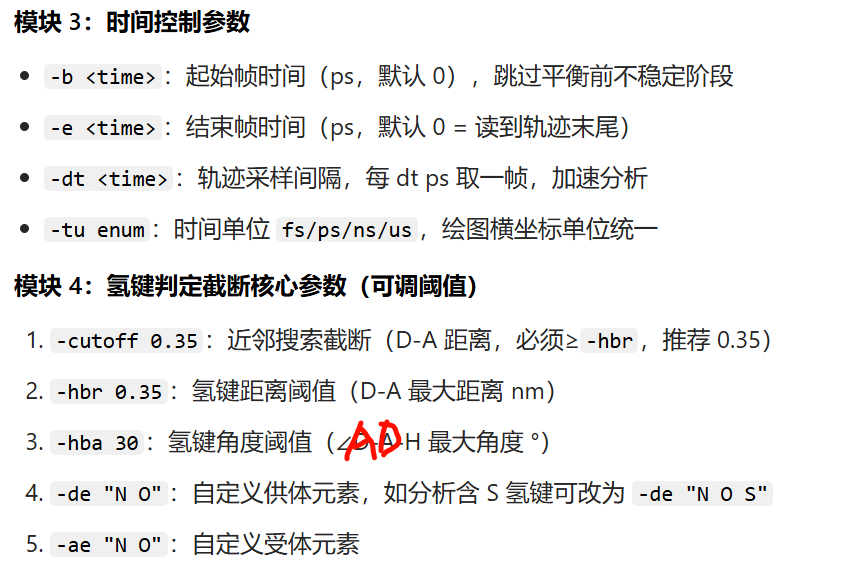
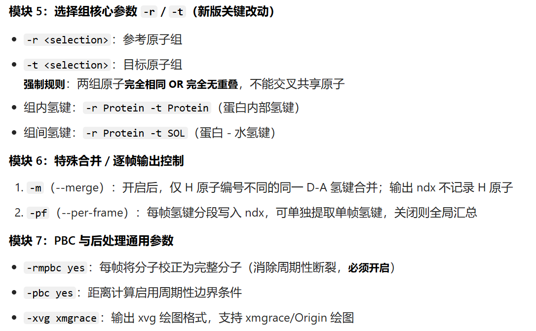
运行后交互式弹窗让你输入两组原子选择:-r参考组、-t目标组 。
蛋白主链内部氢键(MainChain+H)
按照教程,我们先计算主链骨架内的氢键数目:
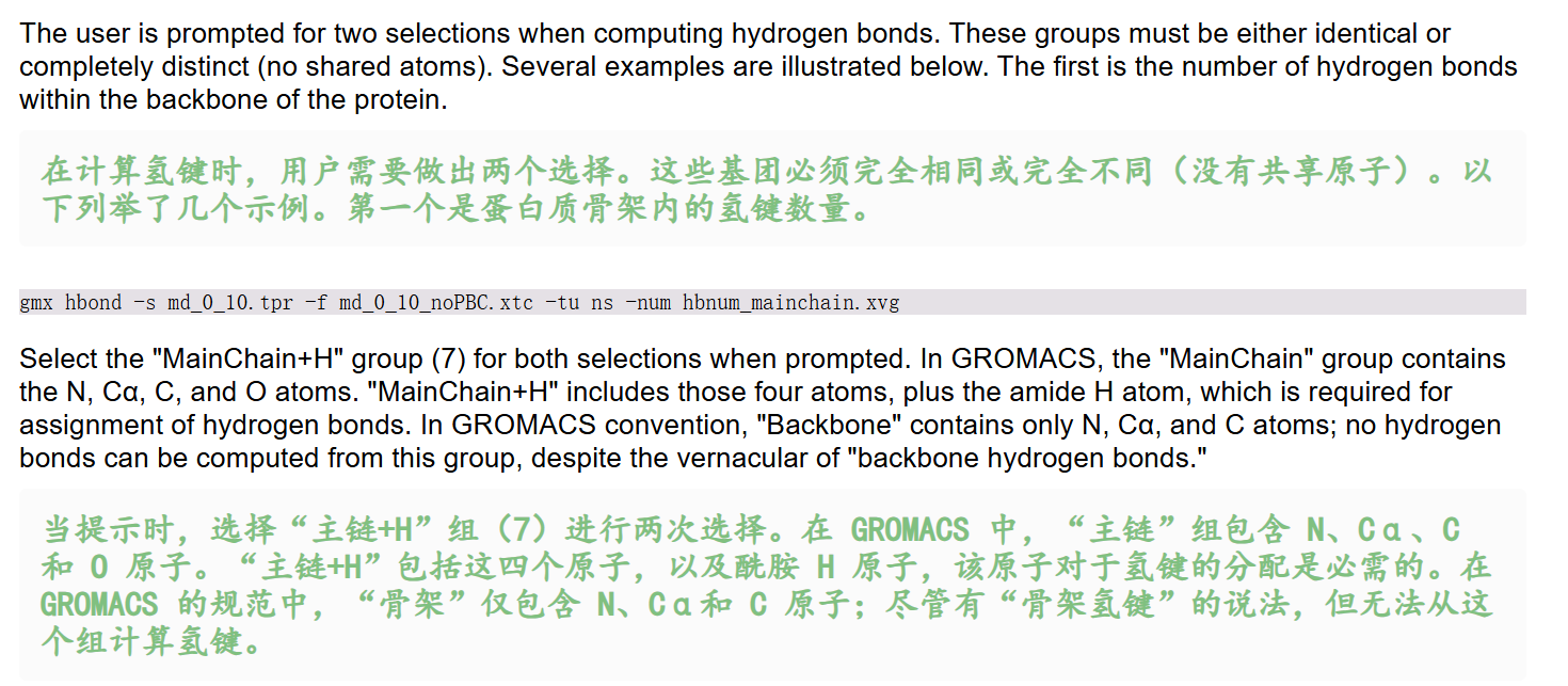
python
gmx hbond -s md_0_10.tpr -f md_0_10_noPBC.xtc -tu ns -num hbnum_mainchain.xvg输出是-num的文件
- 运行后两次选择均输入:
MainChain+H(组7) - 关键知识点:
MainChain仅含N/Cα/C/O,无H,无法计算氢键;MainChain+H包含酰胺H,是统计主链氢键唯一合法组;
- 结果意义:主链氢键数量反映蛋白二级结构(α螺旋/β折叠)稳定性。
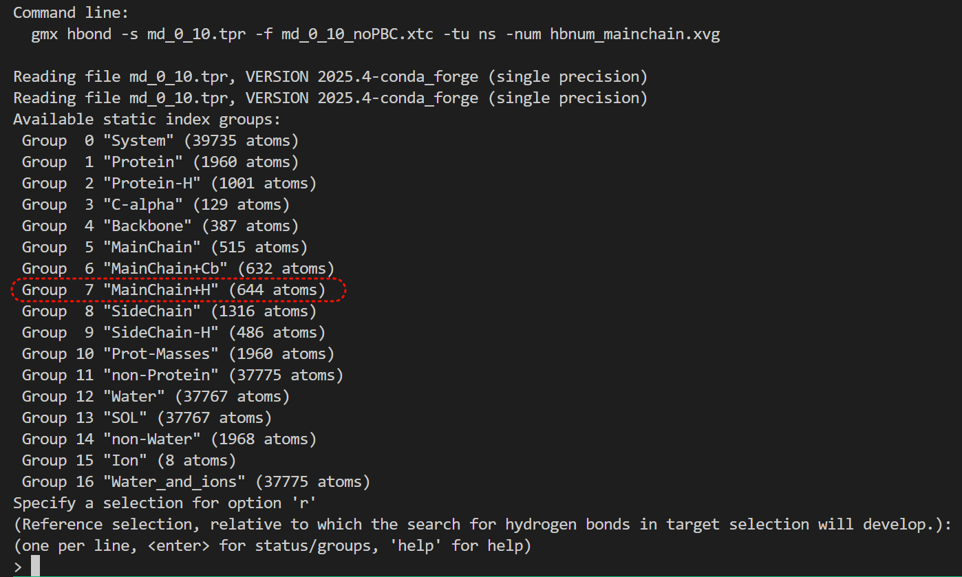
注意参考r和目标t分组,我们都选mainchain+H
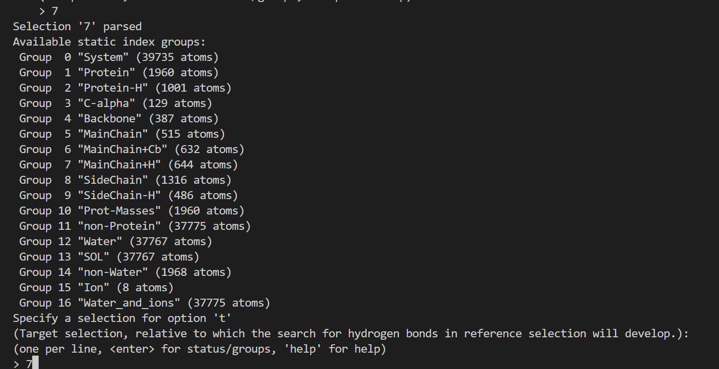
核心部分日志如下
python
# 校验两组选择(-r 和 -t 都选了 MainChain+H)的原子重叠;两组完全一样,代表计算组内氢键(蛋白主链内部氢键),
# 每组均 644 个主链含氢原子,符合 hbond "两组完全相同" 的规则
Checking for overlap in atoms between MainChain+H (644 atoms) and MainChain+H (644 atoms)
# 该主链基团里:257 个氢键受体原子(羰基 O 为主),127 个氢键供体原子(酰胺 N-H 的 N)
Selection 'MainChain+H' has 257 acceptors and 127 donors.
Last frame       1000 time   10.000
# 一共读取分析了 1001 帧轨迹,覆盖到模拟时间 10000 ps(即 10 ns),氢键统计全部计算完成
Analyzed 1001 frames, last time 10000.000

++++ PLEASE READ AND CITE THE FOLLOWING REFERENCE ++++
S. Gorelov, A. Titov, O. Tolicheva, A. Konevega, A. Shvetsov
Determination of Hydrogen Bonds in GROMACS: A New Implementation to Overcome
Memory Limitation
Journal of Chemical Information and Modeling (2024)
DOI: 10.1021/acs.jcim.3c02087
-------- -------- --- Thank You --- -------- --------
蛋白侧链内部氢键(SideChain)
这里关于蛋白质主链以及侧链上的氢键的介绍,
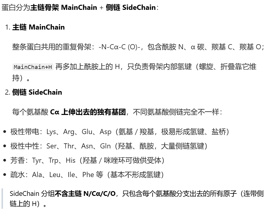
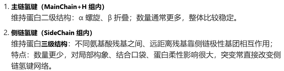
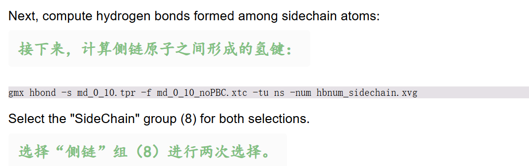
bash
gmx hbond -s md_0_10.tpr -f md_0_10_noPBC.xtc -tu ns -num hbnum_sidechain.xvg- 两次选择均输入:
SideChain(组8) - 结果意义:侧链氢键维持三级结构,数量更少。
python
# 校验两组原子,两次都选了 SideChain 侧链组,每组共 1316 个侧链原子;两组原子完全重合,代表计算侧链内部氢键,符合 gmx hbond 组内氢键的选择规则
Checking for overlap in atoms between SideChain (1316 atoms) and SideChain (1316 atoms)
# 整个蛋白侧链里:
# 121 个氢键受体原子(侧链羰基氧、羟基氧、咪唑氮等)
# 83 个氢键供体原子(侧链 N-H、O-H 上的氢连接原子)
Selection 'SideChain' has 121 acceptors and 83 donors.

Back Off! I just backed up hbond.ndx to ./#hbond.ndx.1#
Last frame       1000 time   10.000
# 完整分析了 1001 帧轨迹,覆盖 0~10000 ps(10 ns)全部模拟数据,侧链氢键计算正常跑完
Analyzed 1001 frames, last time 10000.000
蛋白-水分子间氢键(溶剂化氢键)
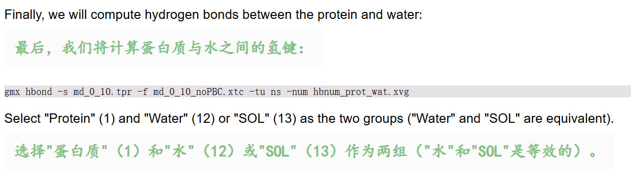
bash
gmx hbond -s md_0_10.tpr -f md_0_10_noPBC.xtc -tu ns -num hbnum_prot_wat.xvg- 第一次选
Protein(1),第二次选Water/SOL(12/13,二者等价) - 结果意义:氢键数量反映蛋白表面亲水程度、溶剂化壳层强弱
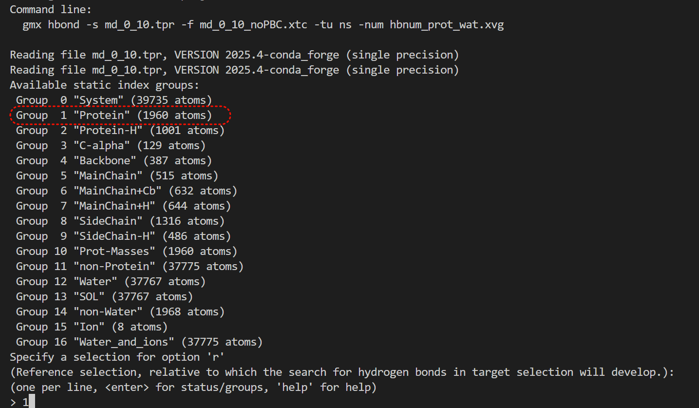
先选protein,再选溶剂水
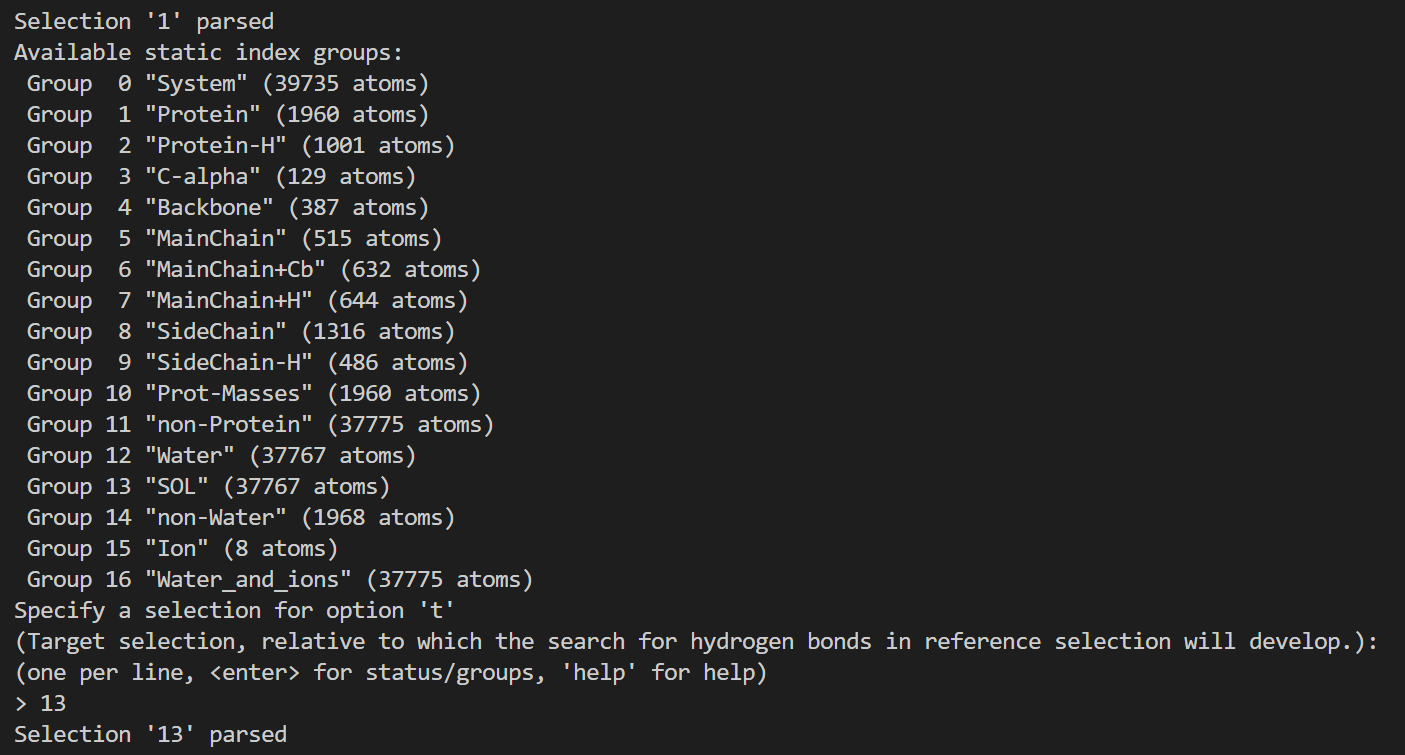
完整输出日志信息如下
python
# 校验两组原子:蛋白共 1960 个原子、水分子 SOL 共 37767 个原子,两组无重叠,用于计算蛋白 - 水分子间氢键
Checking for overlap in atoms between Protein (1960 atoms) and SOL (37767 atoms)
# 蛋白上有 378 个氢键受体、210 个氢键供体
# 378=257+121,210=127+83,其实就是将前面蛋白质中主链和侧链加起来
Selection 'Protein' has 378 acceptors and 210 donors.
# 水分子中氧为受体、氢为供体,各 12589 个
Selection 'SOL' has 12589 acceptors and 12589 donors.

Back Off! I just backed up hbond.ndx to ./#hbond.ndx.2#
Last frame       1000 time   10.000
# 完整分析全部 1001 帧(0~10000 ps / 10 ns),蛋白 - 水氢键计算顺利跑完,无报错
Analyzed 1001 frames, last time 10000.000
然后一起绘制在一起
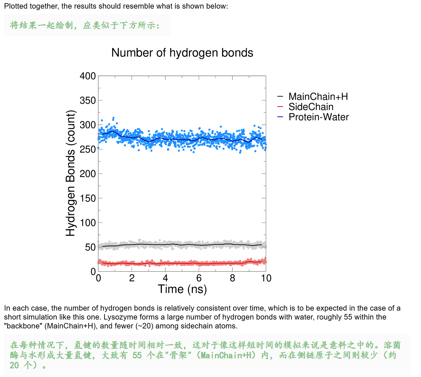
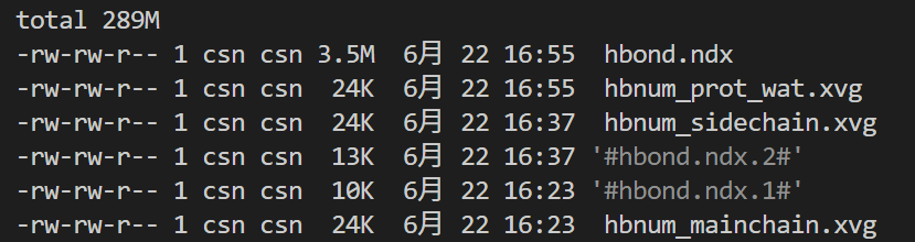
我们可以看到每一次生成输出的文件,除了xvg之外,就是hbond的ndx索引文件(3份备份)
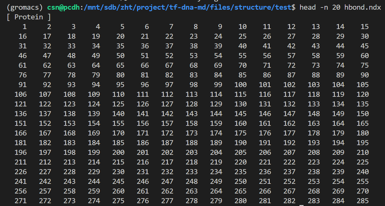
然后我们再可视化一下这些xvg文件,
python
gmxplot multi-compare hbnum_mainchain.xvg hbnum_sidechain.xvg hbnum_prot_wat.xvg 
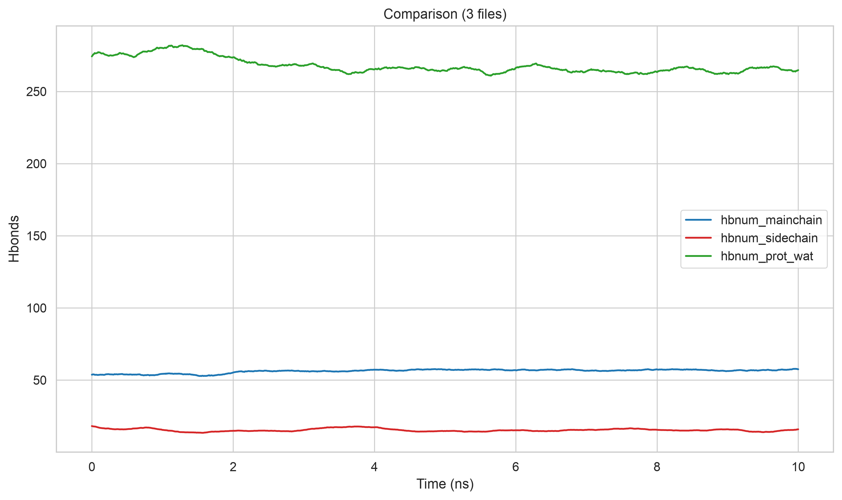
基本上效果是差不多的。
其实说到这里,目前圈内有很多分析氢键的更加现代化的工具,
不再是数氢键数目,而是去定义和分析氢键网络,其空间分布等等。
参考:https://mp.weixin.qq.com/s/oEztQI3mzVkbS-RPeyR6bw
https://mp.weixin.qq.com/s/g4tnDgELcpwmyEQjD65A-g
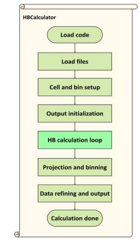
项目仓库地址:https://github.com/yuxiangwang321/HydrogenBondCalculator(可以看到基本上是2-3年前的了)
论坛地址:https://groups.google.com/g/tools-from-yuxiangwang321