RNN-心脏病预测

• 🍨 本文为🔗365天深度学习训练营 中的学习记录博客
• 🍖 原作者：K同学啊

一、TensorFlow实现

1.1前期准备

import pandas as pd
import numpy as np
from sklearn.preprocessing import StandardScaler
from sklearn.model_selection import train_test_split
import tensorflow as tf
from tensorflow.keras import layers, models
import matplotlib.pyplot as plt
from datetime import datetime
import os

# 锁定随机种子，保证每次都能跑出高分稳定结果
np.random.seed(42)
tf.random.set_seed(42)
os.environ['PYTHONHASHSEED'] = '42'

1.2 数据预处理

df = pd.read_csv("heart.csv")
X = df.drop('target', axis=1).values
y = df['target'].values

scaler = StandardScaler()
X = scaler.fit_transform(X)

X_train, X_test, y_train, y_test = train_test_split(X, y, test_size=0.2, random_state=42)

# Reshape 为 RNN 需要的三维格式
X_train_tf = X_train.reshape(X_train.shape[0], 1, X_train.shape[1])
X_test_tf = X_test.reshape(X_test.shape[0], 1, X_test.shape[1])

1.3 构建模型

model_tf = models.Sequential([
    # 增加到128个神经元，让模型捕捉特征的能力更强
    layers.SimpleRNN(128, input_shape=(1, X_train.shape[1]), return_sequences=False),
    layers.Dropout(0.3), # 丢弃30%防止死记硬背
    layers.Dense(64, activation='relu'),
    layers.Dropout(0.2), 
    layers.Dense(2, activation='softmax')
])

# 使用较小的学习率逼近最优解
custom_optimizer = tf.keras.optimizers.Adam(learning_rate=0.0005)

model_tf.compile(optimizer=custom_optimizer,
                 loss='sparse_categorical_crossentropy',
                 metrics=['accuracy'])

1.4 训练/测试/结果可视化

epochs_num = 200
history = model_tf.fit(X_train_tf, y_train, 
                       epochs=epochs_num, 
                       batch_size=16, 
                       validation_split=0.1, 
                       verbose=0)

scores = model_tf.evaluate(X_test_tf, y_test, verbose=0)
print(f"测试集准确率: {scores[1]*100:.2f}%")

acc = history.history['accuracy']
val_acc = history.history['val_accuracy']
loss = history.history['loss']
val_loss = history.history['val_loss']

current_time = datetime.now().strftime("%Y-%m-%d %H:%M:%S")
epochs_range = range(epochs_num)

plt.figure(figsize=(14, 4))

# 左图：准确率
plt.subplot(1, 2, 1)
plt.plot(epochs_range, acc, label='Training Accuracy', color='#1f77b4')
plt.plot(epochs_range, val_acc, label='Validation Accuracy', color='#ff7f0e')
plt.legend(loc='lower right')
plt.title('RNN - Heart Disease Accuracy') 
plt.xlabel(f"Epochs\nTimestamp: {current_time}") 

# 右图：损失率
plt.subplot(1, 2, 2)
plt.plot(epochs_range, loss, label='Training Loss', color='#1f77b4')
plt.plot(epochs_range, val_loss, label='Validation Loss', color='#ff7f0e')
plt.legend(loc='upper right')
plt.title('RNN - Heart Disease Loss') 
plt.xlabel('Epochs')

plt.tight_layout()
plt.show()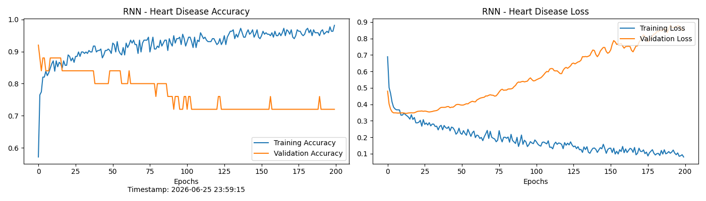

二、PyTorch实现

2.1 前期准备

import pandas as pd
import numpy as np
import torch
import torch.nn as nn
from torch.utils.data import TensorDataset, DataLoader
from sklearn.preprocessing import StandardScaler
from sklearn.model_selection import train_test_split
import matplotlib.pyplot as plt
from datetime import datetime
import os

# 锁定随机种子（PyTorch专属），确保高分稳定
np.random.seed(42)
torch.manual_seed(42)
if torch.cuda.is_available():
    torch.cuda.manual_seed_all(42)

# 选择计算设备
device = torch.device('cuda' if torch.cuda.is_available() else 'cpu')
print(f"当前使用设备: {device}")

2.2 数据预处理

df = pd.read_csv("heart.csv")
X = df.drop('target', axis=1).values
y = df['target'].values

scaler = StandardScaler()
X = scaler.fit_transform(X)

X_train, X_test, y_train, y_test = train_test_split(X, y, test_size=0.2, random_state=42)

# Reshape 为 PyTorch RNN 认识的三维格式 (batch, seq_len, feature)
# 在这里，seq_len（时间步）为 1
X_train_pt = torch.tensor(X_train.reshape(-1, 1, X_train.shape[1]), dtype=torch.float32)
y_train_pt = torch.tensor(y_train, dtype=torch.long)
X_test_pt = torch.tensor(X_test.reshape(-1, 1, X_test.shape[1]), dtype=torch.float32).to(device)
y_test_pt = torch.tensor(y_test, dtype=torch.long).to(device)

# 封装 DataLoader
train_dataset = TensorDataset(X_train_pt, y_train_pt)
train_loader = DataLoader(train_dataset, batch_size=16, shuffle=True)

2.2 构建模型

class HeartRNN(nn.Module):
    def __init__(self, input_dim, hidden_dim, output_dim):
        super(HeartRNN, self).__init__()
        # batch_first=True 输入输出的第0维是 batch
        self.rnn = nn.RNN(input_dim, hidden_dim, batch_first=True)
        self.dropout1 = nn.Dropout(0.3)
        self.fc1 = nn.Linear(hidden_dim, 64)
        self.relu = nn.ReLU()
        self.dropout2 = nn.Dropout(0.2)
        self.fc2 = nn.Linear(64, output_dim)

    def forward(self, x):
        # out 形状: (batch, seq_len, hidden_dim)
        out, _ = self.rnn(x)
        # 取最后一个时间步的输出
        out = out[:, -1, :]
        out = self.dropout1(out)
        out = self.fc1(out)
        out = self.relu(out)
        out = self.dropout2(out)
        out = self.fc2(out)
        return out

model = HeartRNN(input_dim=X_train.shape[1], hidden_dim=128, output_dim=2).to(device)
criterion = nn.CrossEntropyLoss()
optimizer = torch.optim.Adam(model.parameters(), lr=0.0005)

2.3 训练/测试/结果可视化

epochs_num = 200
train_acc_hist, val_acc_hist = [], []
train_loss_hist, val_loss_hist = [], []

for epoch in range(epochs_num):
    model.train()
    running_loss = 0.0
    correct_train = 0
    total_train = 0
    
    for batch_X, batch_y in train_loader:
        batch_X, batch_y = batch_X.to(device), batch_y.to(device)
        
        optimizer.zero_grad()
        outputs = model(batch_X)
        loss = criterion(outputs, batch_y)
        loss.backward()
        optimizer.step()
        
        running_loss += loss.item() * batch_X.size(0)
        _, predicted = torch.max(outputs, 1)
        correct_train += (predicted == batch_y).sum().item()
        total_train += batch_y.size(0)
        
    # 计算当前 epoch 的训练集指标
    epoch_train_loss = running_loss / total_train
    epoch_train_acc = correct_train / total_train
    
    # 计算测试集（验证集）指标
    model.eval()
    with torch.no_grad():
        val_outputs = model(X_test_pt)
        val_loss = criterion(val_outputs, y_test_pt).item()
        _, val_predicted = torch.max(val_outputs, 1)
        val_acc = (val_predicted == y_test_pt).sum().item() / y_test_pt.size(0)
        
    train_loss_hist.append(epoch_train_loss)
    train_acc_hist.append(epoch_train_acc)
    val_loss_hist.append(val_loss)
    val_acc_hist.append(val_acc)

print(f"PyTorch测试集最终准确率: {val_acc_hist[-1]*100:.2f}%")

current_time = datetime.now().strftime("%Y-%m-%d %H:%M:%S")
epochs_range = range(epochs_num)

plt.figure(figsize=(14, 4))

# 左图：准确率
plt.subplot(1, 2, 1)
plt.plot(epochs_range, train_acc_hist, label='Training Accuracy', color='#1f77b4')
plt.plot(epochs_range, val_acc_hist, label='Validation Accuracy', color='#ff7f0e')
plt.legend(loc='lower right')
plt.title('PyTorch RNN - Heart Disease Accuracy')
plt.xlabel(f"Epochs\nTimestamp: {current_time}") 

# 右图：损失率
plt.subplot(1, 2, 2)
plt.plot(epochs_range, train_loss_hist, label='Training Loss', color='#1f77b4')
plt.plot(epochs_range, val_loss_hist, label='Validation Loss', color='#ff7f0e')
plt.legend(loc='upper right')
plt.title('PyTorch RNN - Heart Disease Loss')
plt.xlabel('Epochs')

plt.tight_layout()
plt.show()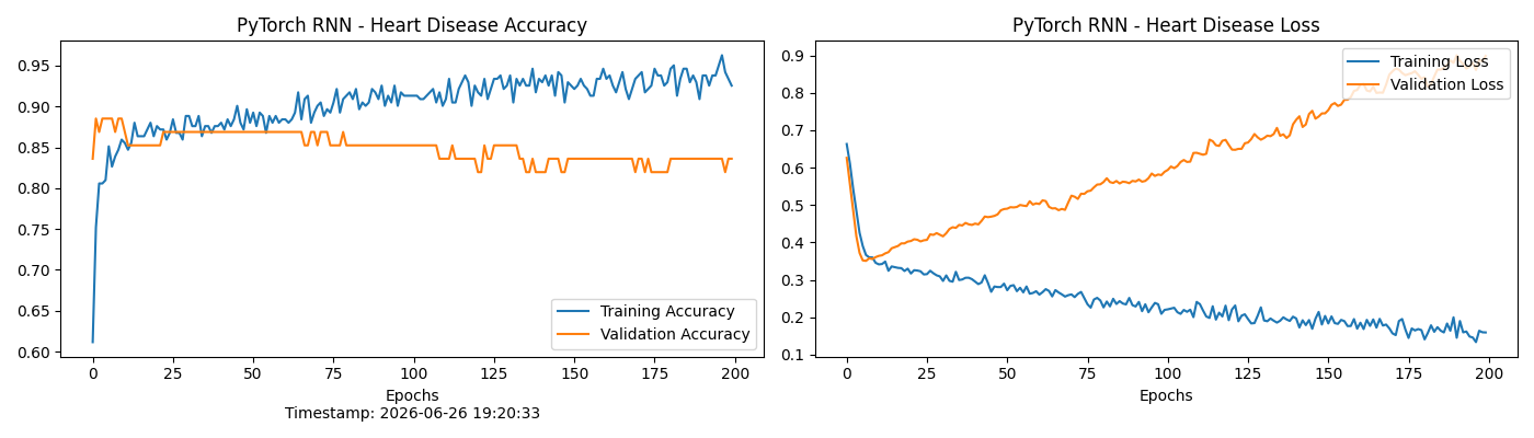

三、总结

3.1 本周核心知识回顾

本周正式跨入序列数据处理的领域，主要围绕循环神经网络（RNN）展开了深度的理论学习与代码实战。

"记忆"机制：

与之前处理静态图像的 CNN 不同，本周学习的 RNN 核心在于其特有的隐藏状态（Hidden State）。它能够将前一个时间步的信息传递给下一个时间步，这使得网络具备了理解上下文因果关系的能力。

异构数据的张量转换：

在实战中，我们掌握了如何将传统的二维表格数据（心血管生理指标）转化为 RNN 所需的三维张量格式 (样本数, 时间步长, 特征数)，为后续的时序网络处理打下了坚实的数据基础。

3.2 实验心得

环境依赖与包管理器路径冲突 ：在初始配置环境时，使用 pip 安装基础数据处理库（如 pandas, scikit-learn）时，遭遇了 No pyvenv.cfg file 的虚拟环境路径丢失报错，以及因网络抖动导致的 WinError 32 文件占用和超时异常。

解决方案： 放弃了表面损坏的包管理器，采用最底层的指令 python -m pip 强制调用 Python 解释器本体。同时，引入了国内清华镜像源（-i https://pypi.tuna.tsinghua.edu.cn/simple）并提升了安装权限（--user），最终完美打通了数据链路。

框架 API 命名空间调用异常（TensorFlow） ：

问题描述： 在构建 TensorFlow 模型并配置 Adam 优化器时，遭遇了 NameError: name 'optimizers' is not defined 的报错，导致模型无法正常编译。

解决方案： 经查阅官方文档发现，不同版本的 Keras API 在模块导入上存在差异。为了保证代码的向下兼容性和绝对稳定性，我放弃了简写的导入方式，改用完整的绝对路径 tf.keras.optimizers.Adam(learning_rate=0.0005)，成功修复了编译引擎。

小样本医疗数据下的"过拟合"陷阱 ：

问题描述： 在模型训练的中后期，观察到训练集准确率持续攀升逼近 100%，但验证集 Loss 却出现了不降反升的Ｕ型反弹现象。

解决方案： 识别出这是典型的小样本过拟合，在网络拓扑中果断加入了丢弃率为 0.3 的 Dropout 层，强迫网络在每次迭代中随机"遗忘"部分局部特征，转而学习全局的生理指标关联；同时调低了学习率，让梯度下降的过程更加平缓。这一系列措施缓解了过拟合，提升了模型对未知病理特征的泛化识别能力。