TensorFlow

核心概念

TensorFlow 是一个数学计算的工具箱，专门为机器学习任务而设计，让开发者能够轻松地构建从简单线性回归到复杂神经网络的各种模型。

TensorFlow 是由 Google 开发的开源机器学习框架，用于构建和训练各种机器学习和深度学习模型。

TensorFlow 名字来源于其核心概念：Tensor（张量） 和 Flow（流动），表示数据以张量的形式在计算图中流动。

核心概念

• 张量(Tensor): 多维数组，是 TensorFlow 中的基本数据单位
• 计算图(Computational Graph): 描述数据(Tensor)流动(Flow)的有向图
• 会话(Session): 执行计算图的运行时环境

安装：

# 确保在虚拟环境中
pip install tensorflow

# 验证安装
import tensorflow as tf;
print('TensorFlow version:', tf.__version__)

TensorFlow version: 2.21.0

张量（Tensor）

张量是 TensorFlow 中最基本的数据结构，可以理解为多维数组的泛化概念。从数学角度来说，张量是一个可以用来表示在一些矢量、标量和其他张量之间的线性关系的多线性函数。在机器学习中，几乎所有数据最终都会被表示为张量形式进行处理。

张量的基本特性

1. 数据类型(dtype)：每个张量都有特定的数据类型，如tf.float32、tf.int64等
2. 形状(shape)：表示张量每个维度的大小，如(2,3)表示2行3列的矩阵
3. 设备位置(device)：指示张量存储在CPU还是GPU上

简单类比：

• 标量（0维张量）scalar ：一个数字如 5，tf.constant(5)
• 向量（1维张量）vector ：一列数字，如 [1, 2, 3, 4]，tf.constant([1,2,3,4])
• 矩阵（2维张量）matrix ：数字的表格，如 [[1, 2], [3, 4]],tf.constant(\[1,2,3,4])
• 3维张量 ：数字的立方体，如彩色图像（高×宽×颜色通道），tf.ones((2,3,4)) 表示2个3×4的矩阵
• 更高维张量：例如视频数据（时间×高×宽×颜色通道）

创建张量的常用方法

1. 从Python列表/NumPy数组创建

# 从Python列表创建
tensor_from_list = tf.constant([[1, 2], [3, 4]])

# 从NumPy数组创建
numpy_array = np.array([[5, 6], [7, 8]])
tensor_from_numpy = tf.constant(numpy_array)

2. 创建特殊值张量

# 全零张量
zeros = tf.zeros((2, 3))  # 2行3列的全0矩阵

# 全一张量
ones = tf.ones((3, 2))    # 3行2列的全1矩阵

# 单位矩阵
eye = tf.eye(3)           # 3×3的单位矩阵

# 填充特定值
filled = tf.fill((2, 2), 7)  # 2×2矩阵，所有元素为7

3. 创建随机张量

# 均匀分布随机数
uniform = tf.random.uniform((2, 2), minval=0, maxval=1)

# 正态分布随机数
normal = tf.random.normal((3, 3), mean=0, stddev=1)

# 随机排列
shuffled = tf.random.shuffle(tf.constant([1, 2, 3, 4, 5]))

张量的基本操作

1. 数学运算

a = tf.constant([[1, 2], [3, 4]])
b = tf.constant([[5, 6], [7, 8]])

# 逐元素加法
add = tf.add(a, b)        # 或使用运算符重载 a + b

# 逐元素乘法
mul = tf.multiply(a, b)   # 或 a * b

# 矩阵乘法
matmul = tf.matmul(a, b)  # 或 a @ b

# 其他数学运算
sqrt = tf.sqrt(tf.cast(a, tf.float32))  # 平方根(需要转换为浮点型)

2. 形状操作

tensor = tf.constant([[1, 2, 3], [4, 5, 6]])

# 获取形状
shape = tensor.shape  # 返回 (2, 3)

# 改变形状(reshape)
reshaped = tf.reshape(tensor, (3, 2))  # 变为3行2列

# 转置(transpose)
transposed = tf.transpose(tensor)  # 变为3行2列

# 扩展维度(expand_dims)
expanded = tf.expand_dims(tensor, axis=0)  # 形状从(2,3)变为(1,2,3)

3. 索引与切片

tensor = tf.constant([[1, 2, 3], [4, 5, 6], [7, 8, 9]])

# 获取单个元素
elem = tensor[1, 2]  # 获取第2行第3列的元素(值为6)

# 切片操作
row = tensor[1, :]    # 获取第2行所有元素 [4,5,6]
col = tensor[:, 1]    # 获取第2列所有元素 [2,5,8]
sub = tensor[0:2, 1:] # 获取第1-2行，第2-3列 [[2,3],[5,6]]

张量的广播机制

广播(Broadcasting)是TensorFlow中处理不同形状张量运算的重要机制，它自动扩展较小的张量以匹配较大张量的形状。

广播规则

1. 从最后一个维度开始向前比较
2. 两个维度要么相等，要么其中一个为1，要么其中一个不存在
3. 在缺失或为1的维度上进行复制扩展

# 向量(3,)与标量()相加
a = tf.constant([1, 2, 3])
b = tf.constant(2)
c = a + b  # 结果为[3,4,5]，b被广播为[2,2,2]

# 矩阵(3,1)与向量(3,)相加
d = tf.constant([[1], [2], [3]])
e = tf.constant([10, 20, 30])
f = d + e  # d被广播为[[1,1,1],[2,2,2],[3,3,3]]
           # 结果为[[11,21,31],[12,22,32],[13,23,33]]

张量的聚合操作

常用聚合函数

tensor = tf.constant([[1, 2, 3], [4, 5, 6]])

# 求和
sum_all = tf.reduce_sum(tensor)        # 所有元素求和 → 21
sum_axis0 = tf.reduce_sum(tensor, 0)  # 沿第0维(行)求和 → [5,7,9]
sum_axis1 = tf.reduce_sum(tensor, 1)  # 沿第1维(列)求和 → [6,15]

# 求均值
mean_all = tf.reduce_mean(tensor)      # 所有元素均值 → 3.5

# 最大值/最小值
max_val = tf.reduce_max(tensor)        # 最大值 → 6
min_val = tf.reduce_min(tensor)       # 最小值 → 1

# 逻辑运算
any_true = tf.reduce_any(tensor > 4)   # 是否有元素>4 → True
all_true = tf.reduce_all(tensor > 0)   # 是否所有元素>0 → True

练习1：创建和操作张量

# 1. 创建一个3×3的随机矩阵，元素值在0-10之间
random_matrix = tf.random.uniform((3, 3), minval=0, maxval=10, dtype=tf.int32)

# 2. 计算该矩阵的转置
transposed_matrix = tf.transpose(random_matrix)

# 3. 计算矩阵与转置矩阵的乘积
product = tf.matmul(random_matrix, transposed_matrix)

# 4. 计算乘积矩阵的对角线元素之和
diag_sum = tf.reduce_sum(tf.linalg.diag_part(product))

练习2：广播机制应用

# 1. 创建一个4×1的矩阵和一个1×4的向量
matrix = tf.constant([[1], [2], [3], [4]])
vector = tf.constant([10, 20, 30, 40])

# 2. 利用广播机制计算它们的和
broadcast_sum = matrix + vector

# 3. 验证结果的形状和值
print("形状:", broadcast_sum.shape)  # 应为(4,4)
print("结果:", broadcast_sum.numpy())

TensorFlow 高级 API - Keras

Keras 是一个用 Python 编写的高级神经网络 API，为TensorFlow的代码提供了新的风格和设计模式，大大提升了TF代码的简洁性和复用性，官方也推荐使用tf.keras来进行模型设计和开发。

Keras 核心概念

1. 模型 (Model)

Keras 的核心数据结构是模型，模型是组织神经网络层的方式。Keras 提供了两种主要的模型：

• Sequential 模型：层的线性堆叠
• Functional API：构建复杂模型的有向无环图

2. 层 (Layer)

层是 Keras 的基本构建块，每个层接收输入数据，进行某种计算后输出结果。Keras 提供了多种预定义层：

• 核心层：Dense, Activation, Dropout 等
• 卷积层：Conv2D, MaxPooling2D 等
• 循环层：LSTM, GRU 等
• 其他：Embedding, BatchNormalization 等

3. 激活函数 (Activation Function)

激活函数决定神经元的输出，常用的有：

• ReLU (Rectified Linear Unit)
• Sigmoid
• Tanh
• Softmax (多分类问题)

Keras 基本工作流程

1. 定义模型

from tensorflow.keras.models import Sequential
from tensorflow.keras.layers import Dense

model = Sequential([
    Dense(64, activation='relu', input_shape=(784,)),
    Dense(64, activation='relu'),
    Dense(10, activation='softmax')
])

2. 编译模型

model.compile(optimizer='adam',
              loss='categorical_crossentropy',
              metrics=['accuracy'])

3. 训练模型

model.fit(x_train, y_train,
          epochs=5,
          batch_size=32)

4. 评估模型

loss_and_metrics = model.evaluate(x_test, y_test, batch_size=128)

5. 进行预测

classes = model.predict(x_test, batch_size=128)

Keras 常用层详解

1. Dense 全连接层

Dense(units,

activation=None,

use_bias=True,

kernel_initializer='glorot_uniform',

bias_initializer='zeros')

• units：正整数，输出空间的维度
• activation：激活函数
• use_bias：是否使用偏置向量
• kernel_initializer：权重矩阵的初始化器
• bias_initializer：偏置向量的初始化器

2. Conv2D 二维卷积层

Conv2D(filters,

kernel_size,

strides=(1, 1),

padding='valid',

activation=None)

• filters：卷积核的数目
• kernel_size：卷积核的尺寸
• strides：卷积步长
• padding：填充方式 ('valid' 或 'same')

3. LSTM 长短期记忆网络层

LSTM(units,

activation='tanh',

recurrent_activation='hard_sigmoid',

return_sequences=False)

• units：正整数，输出空间的维度
• activation：激活函数
• recurrent_activation：循环步的激活函数
• return_sequences：是否返回完整序列

Keras 实践示例：MNIST 手写数字识别

from tensorflow.keras.datasets import mnist
from tensorflow.keras.models import Sequential
from tensorflow.keras.layers import Dense, Dropout, Flatten
from tensorflow.keras.layers import Conv2D, MaxPooling2D
from tensorflow.keras.utils import to_categorical

# 加载数据
(x_train, y_train), (x_test, y_test) = mnist.load_data()

# 数据预处理
x_train = x_train.reshape(60000, 28, 28, 1).astype('float32') / 255
x_test = x_test.reshape(10000, 28, 28, 1).astype('float32') / 255
y_train = to_categorical(y_train, 10)
y_test = to_categorical(y_test, 10)

# 构建模型
model = Sequential([
    Conv2D(32, kernel_size=(3, 3), activation='relu', input_shape=(28, 28, 1)),
    Conv2D(64, (3, 3), activation='relu'),
    MaxPooling2D(pool_size=(2, 2)),
    Dropout(0.25),
    Flatten(),
    Dense(128, activation='relu'),
    Dropout(0.5),
    Dense(10, activation='softmax')
])

# 编译模型
model.compile(loss='categorical_crossentropy',
              optimizer='adam',
              metrics=['accuracy'])

# 训练模型
model.fit(x_train, y_train,
          batch_size=128,
          epochs=12,
          verbose=1,
          validation_data=(x_test, y_test))

# 评估模型
score = model.evaluate(x_test, y_test, verbose=0)
print('Test loss:', score[0])
print('Test accuracy:', score[1])

输出

Epoch 1/12
469/469 ━━━━━━━━━━━━━━━━━━━━ 39s 64ms/step - accuracy: 0.9270 - loss: 0.2392 - val_accuracy: 0.9835 - val_loss: 0.0482
Epoch 2/12
469/469 ━━━━━━━━━━━━━━━━━━━━ 30s 64ms/step - accuracy: 0.9754 - loss: 0.0833 - val_accuracy: 0.9879 - val_loss: 0.0373
Epoch 3/12
469/469 ━━━━━━━━━━━━━━━━━━━━ 30s 63ms/step - accuracy: 0.9814 - loss: 0.0621 - val_accuracy: 0.9893 - val_loss: 0.0338
Epoch 4/12
469/469 ━━━━━━━━━━━━━━━━━━━━ 30s 63ms/step - accuracy: 0.9844 - loss: 0.0518 - val_accuracy: 0.9894 - val_loss: 0.0290
Epoch 5/12
469/469 ━━━━━━━━━━━━━━━━━━━━ 30s 63ms/step - accuracy: 0.9869 - loss: 0.0422 - val_accuracy: 0.9908 - val_loss: 0.0290
Epoch 6/12
469/469 ━━━━━━━━━━━━━━━━━━━━ 29s 63ms/step - accuracy: 0.9879 - loss: 0.0387 - val_accuracy: 0.9910 - val_loss: 0.0281
Epoch 7/12
469/469 ━━━━━━━━━━━━━━━━━━━━ 30s 65ms/step - accuracy: 0.9889 - loss: 0.0339 - val_accuracy: 0.9918 - val_loss: 0.0269
Epoch 8/12
469/469 ━━━━━━━━━━━━━━━━━━━━ 30s 63ms/step - accuracy: 0.9904 - loss: 0.0299 - val_accuracy: 0.9907 - val_loss: 0.0262
Epoch 9/12
469/469 ━━━━━━━━━━━━━━━━━━━━ 30s 63ms/step - accuracy: 0.9910 - loss: 0.0273 - val_accuracy: 0.9920 - val_loss: 0.0269
Epoch 10/12
469/469 ━━━━━━━━━━━━━━━━━━━━ 30s 63ms/step - accuracy: 0.9918 - loss: 0.0243 - val_accuracy: 0.9916 - val_loss: 0.0300
Epoch 11/12
469/469 ━━━━━━━━━━━━━━━━━━━━ 31s 66ms/step - accuracy: 0.9920 - loss: 0.0239 - val_accuracy: 0.9912 - val_loss: 0.0317
Epoch 12/12
469/469 ━━━━━━━━━━━━━━━━━━━━ 34s 72ms/step - accuracy: 0.9934 - loss: 0.0206 - val_accuracy: 0.9918 - val_loss: 0.0272
Test loss: 0.027172742411494255
Test accuracy: 0.9918000102043152

数学学习案例

梯度下降算法理解

一元函数一阶导数就是该函数的梯度

自动微分（Automatic Differentiation）TensorFlow 使用 GradientTape 来记录运算并自动计算梯度：函数： 解析导数：，验证 x=2 时导数 = 14

x = tf.Variable(2.0)

with tf.GradientTape() as tape:
    y = 3 * x**2 + 2 * x + 1

# 求dy/dx
dy_dx = tape.gradient(y, x)
print(f"计算导数：{dy_dx.numpy()}")  # 输出14.0
print(f"解析解验证：6*2+2 = {6*2+2}")

多元函数梯度是各偏导组成的梯度向量

二元函数：

偏导数：

梯度为

取 x=1, y=2

x = tf.Variable(1.0)
y = tf.Variable(2.0)

with tf.GradientTape() as tape:
    f = x**2 + 3*x*y + y**3

# 一次性求多个梯度
df_dx, df_dy = tape.gradient(f, [x, y])
print(f"df/dx = {df_dx.numpy()}")  # 2*1+3*2=8
print(f"df/dy = {df_dy.numpy()}")  # 3*1+3*(2^2)=15
# 梯度向量 [8,15]

多元函数：，参数向量

梯度 是损失函数对所有参数的偏导数构成的向量：

梯度下降算法

梯度下降是最小化损失函数的迭代优化算法，广泛用于线性回归、逻辑回归、神经网络。

一句话：沿着损失函数梯度的反方向，一步步更新参数，直到损失最小。

梯度方向 = 函数上升最快的方向，在一维平面函数中即为函数的导数，在二维或多维函数中为 每个参数 的偏导数所构成的向量。

目标：找到损失函数 最小值。它的函数图像如下：

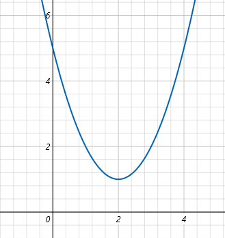
损失函数对应的导数为 ，当然只需要调用 gradient 方法即可得到。

通用梯度下降迭代公式： ，：学习率（learning rate） ，控制每一步走多大。（梯度/导数越大，说明此时前进的步子越大，为了防止迭代步子太大超过极值使用 控制，梯度前加⼀个负号，就意味着朝着梯度相反的⽅向前进！我们在前⽂提到，梯度的⽅向实际就是函数在此点上升最快的⽅向！⽽我们需要朝着下降最快的⽅向⾛，⾃然就是负的梯度的⽅向，所以此处需要加上负号）

极小值点 x=2 手动利用梯度迭代更新参数

x = tf.Variable(0.0) #从0开始找
lr = 0.2  # 学习率
epochs = 30 #迭代30次

for i in range(epochs):
    with tf.GradientTape() as tape:
        y = x**2 - 4*x +5
    grad = tape.gradient(y, x)
    # 梯度下降更新：x = x - lr * grad
    x.assign_sub(lr * grad)
    if i % 5 == 0:
        print(f"迭代{i}, x={x.numpy():.3f}, loss={y.numpy():.3f}")

输出会逐步收敛到 x≈2，loss≈1。

迭代0, x=0.800, loss=5.000
迭代5, x=1.907, loss=1.024
迭代10, x=1.993, loss=1.000
迭代15, x=1.999, loss=1.000
迭代20, x=2.000, loss=1.000
迭代25, x=2.000, loss=1.000

多次复用求导

普通 tape 只能调用一次.gradient()，persistent=True可多次求导

x = tf.Variable(2.0)
with tf.GradientTape(persistent=True) as tape:
    y1 = x ** 2
    y2 = x ** 3

# 多次求梯度
dy1_dx = tape.gradient(y1, x)
dy2_dx = tape.gradient(y2, x)
print(dy1_dx.numpy()) # 4
print(dy2_dx.numpy()) # 12

高阶导数

函数 ，一阶导为： ，二阶导为： ，当 x=3 时：一阶导：27.0, 二阶导：18.0。使用嵌套 GradientTape 实现高阶微分

x = tf.Variable(3.0)
with tf.GradientTape() as tape2:
    with tf.GradientTape() as tape1:
        y = x ** 3
    dy_dx = tape1.gradient(y, x)  # 一阶导
d2y_dx2 = tape2.gradient(dy_dx, x) # 二阶导
print(f"一阶导：{dy_dx.numpy()}, 二阶导：{d2y_dx2.numpy()}")