Matrix Multiplication Performance (矩阵乘法性能)

Matrix Multiplication Performance {矩阵乘法性能}

[1. Introduction](#1. Introduction)
- [1.1. FLOPS and FLOPs](#1.1. FLOPS and FLOPs)
- [1.2. FLOPs and IOPs](#1.2. FLOPs and IOPs)
- [1.3. Frequency (频率) and Hz (赫兹)](#1.3. Frequency (频率) and Hz (赫兹))
- [1.4. FMA, MAC and FLOPs](#1.4. FMA, MAC and FLOPs)
[2. Matrix-Matrix Multiplication](#2. Matrix-Matrix Multiplication)
[3. Math And Memory Bounds (计算瓶颈与内存瓶颈)](#3. Math And Memory Bounds (计算瓶颈与内存瓶颈))
- [3.1. Batch Matrix Multiplication (Batch MatMul)](#3.1. Batch Matrix Multiplication (Batch MatMul))
- [3.2. Arithmetic Intensity](#3.2. Arithmetic Intensity)
- [3.3. GPU Implementation](#3.3. GPU Implementation)
- [3.4. Tensor Core Requirements](#3.4. Tensor Core Requirements)
- [3.5. Typical Tile Dimensions In cuBLAS And Performance](#3.5. Typical Tile Dimensions In cuBLAS And Performance)
[4. Dimension Quantization Effects](#4. Dimension Quantization Effects)
- [4.1. Tile Quantization](#4.1. Tile Quantization)
- [4.2. Wave Quantization](#4.2. Wave Quantization)
References

NVIDIA Deep Learning Performance

https://docs.nvidia.com/deeplearning/performance/index.html

1. Introduction

1.1. FLOPS and FLOPs

https://en.wikipedia.org/wiki/Floating_point_operations_per_second

浮点 (floating-point) 指的是带有小数的数值，浮点运算即是小数的四则运算。

FLOPS (FLoating-point Operations Per Second) - 每秒浮点运算次数

Measures hardware performance (speed)

每秒浮点运算次数 (FLoating-point Operations Per Second, FLOPS) 是每秒所执行的浮点运算次数。

FLOPs (FLoating-point OPerations) - 浮点运算次数

Measures model complexity (quantity)

浮点运算次数 (Floating-point OPerations, FLOPs) 用于衡量计算量或模型复杂度的静态指标。

数学关系

运行时间 (秒) = 模型总计算量 (FLOPs) 硬件实际计算速度 (FLOPS) ∗ 硬件利用率 \text{运行时间 (秒)} = \frac{\text{模型总计算量 (FLOPs)}}{\text{硬件实际计算速度 (FLOPS)} * \text{硬件利用率}} 运行时间 (秒)=硬件实际计算速度 (FLOPS)∗硬件利用率模型总计算量 (FLOPs)

在理想情况下，硬件利用率为 100% 时：

理论运行时间 (秒) = 模型总计算量 (FLOPs) 硬件实际计算速度 (FLOPS) \text{理论运行时间 (秒)} = \frac{\text{模型总计算量 (FLOPs)}}{\text{硬件实际计算速度 (FLOPS)}} 理论运行时间 (秒)=硬件实际计算速度 (FLOPS)模型总计算量 (FLOPs)

硬件不可能时刻保持满载。

International System of Units

https://en.wikipedia.org/wiki/International_System_of_Units

1.2. FLOPs and IOPs

https://rocm.docs.amd.com/projects/rocprofiler-compute/en/docs-6.3.1/conceptual/compute-unit.html

FLOPs (FLoating-point OPerations) - 浮点运算次数

Measures model complexity (quantity)

IOPs (Integer OPerations) - 整数运算次数

Measures model complexity (quantity)

1.3. Frequency (频率) and Hz (赫兹)

The hertz (symbol: Hz) is the unit of frequency in the International System of Units (SI), often described as being equivalent to one event (or cycle) per second.

赫兹是频率的国际单位制单位，表示每一秒周期性事件发生的次数。

1 赫兹 (Hz) 表示事件每一秒发生一次。

Replacement of "cycles per second" by "hertz" in the popular press began in the late 1960s.

大众媒体从 20 世纪 60 年代末开始用 "赫兹" 取代 "每秒周期数"。

The unit of measurement of frequency in the International System of Units (SI) is the hertz, having the symbol Hz.

频率是单位时间内某事件重复发生次数。

设 τ \tau τ 时间内某事件重复发生 n n n 次，则此事件发生的频率为：

f = n τ ( Hz ) f =\frac{n}{\tau} (\text{Hz}) f=τn(Hz)

周期定义为重复事件发生的最小时间间隔，故频率也可以表示为周期 ( T T T) 的倒数：

f = 1 T ( Hz ) f = \frac{1}{T} (\text{Hz}) f=T1(Hz)

1.4. FMA, MAC and FLOPs

MAC (Multiply-Accumulate) - 乘积累加运算

The multiply-accumulate (MAC) or multiply-add (MAD) operation is a common step that computes the product of two numbers and adds that product to an accumulator.

The MAC operation modifies an accumulator a a a:

a ← a + ( b ∗ c ) a \gets a + ( b * c ) a←a+(b∗c)

FMA (Fused Multiply-Add) - 融合乘加运算

When performed with a single rounding, it is called a fused multiply-add (FMA) or fused multiply-accumulate (FMAC).

若一条 MAC 指令在处理浮点数时只有一次的数值修约，则这种指令称为 "融合乘加运算" (fused multiply-add, FMA) 或 "熔合乘法累积运算" (fused multiply-accumulate, FMAC)。

A fused multiply-add (FMA or fmadd) is a floating-point multiply-add operation performed in one step (fused operation), with a single rounding. That is, where an unfused multiply-add would compute the product b ∗ c b * c b∗c, round it to N significant bits, add the result to a, and round back to N significant bits, a fused multiply-add would compute the entire expression a + ( b ∗ c ) a + (b * c) a+(b∗c) to its full precision before rounding the final result down to N significant bits.

非融合乘加的乘积累加运算，处理浮点数时，会先完成 b ∗ c b * c b∗c 的乘积，将其结果数值修约到 N 个比特，然后才将修约后的结果与寄存器 a 的数值相加，再把结果修约到 N 个比特；融合乘加则是先完成 a + b ∗ c a + b * c a+b∗c 的操作，获得最终的完整结果后方才修约到 N 个比特。由于减少了数值修约次数，这种操作可以提高运算结果的精度，以及提高运算效率和速率。

FLOPs (Floating Point Operations) - 浮点运算次数

The total count of floating-point operations (additions, subtractions, multiplications, divisions) required by an algorithm or model.

MAC describes the logical operation (multiply and add), while FMA is the hardware implementation that fuses them together into one clock cycle with higher precision.

1 MAC/FMA is frequently counted as 2 FLOPs (1 for multiplication, 1 for addition).

在硬件算力评估中，1 个 MAC/FMA 指令等于 2 个 FLOPs。

2. Matrix-Matrix Multiplication

https://docs.nvidia.com/deeplearning/performance/dl-performance-matrix-multiplication/index.html

GEMMs (General Matrix Multiplications) are a fundamental building block for many operations in neural networks, for example fully-connected layers, recurrent layers such as RNNs, LSTMs or GRUs, and convolutional layers. In this guide, we describe GEMM performance fundamentals common to understanding the performance of such layers.

GEMM is defined as the operation C = α ∗ A @ B + β ∗ C C = \alpha * A @ B + \beta * C C=α∗A@B+β∗C, with A A A and B B B as matrix inputs, α \alpha α and β \beta β as scalar inputs, and C C C as a pre-existing matrix which is overwritten by the output. A plain matrix product A @ B A @ B A@B is a GEMM with α \alpha α equal to one and β \beta β equal to zero. For example, in the forward pass of a fully-connected layer, the weight matrix would be argument A A A, incoming activations would be argument B B B, and α \alpha α and β \beta β would typically be 1 and 0, respectively. β \beta β can be 1 in some cases, for example, if we're combining the addition of a skip-connection with a linear operation.

3. Math And Memory Bounds (计算瓶颈与内存瓶颈)

Following the convention of various linear algebra libraries (such as BLAS), we will say that matrix A A A is an M × K M \times K M×K matrix, meaning that it has M M M rows and K K K columns. Similarly, B B B and C C C will be assumed to be K × N K \times N K×N and M × N M \times N M×N matrices, respectively.

The product of A A A and B B B has M ∗ N M * N M∗N values, each of which is a dot-product of K-element vectors. Thus, a total of M ∗ N ∗ K M * N * K M∗N∗K fused multiply-adds (FMAs) are needed to compute the product. Each FMA is 2 operations, a multiply and an add, so a total of 2 ∗ M ∗ N ∗ K 2 * M * N * K 2∗M∗N∗K FLOPs are required. For simplicity, we are ignoring the α \alpha α and β \beta β parameters for now; as long as K K K is sufficiently large, their contribution to arithmetic intensity is negligible.

3.1. Batch Matrix Multiplication (Batch MatMul)

Tensor A shape: ( B , M , K ) (B, M, K) (B,M,K)
Tensor B shape: ( B , K , N ) (B, K, N) (B,K,N)
Output Tensor shape: ( B , M , N ) (B, M, N) (B,M,N)

Where:

B B B: Batch size
M M M: Rows of the output matrix
N N N: Columns of the output matrix
K K K: Shared dimension (columns of A A A and rows of B B B).

Every single element in the final ( B , M , N ) (B, M, N) (B,M,N) output tensor is produced by a dot product between a row from tensor A A A (length K K K) and a column from tensor B B B (length K K K).

To compute one dot product of length K K K, the hardware must perform:

K K K multiplications ( a 1 ∗ b 1 , a 2 ∗ b 2 , ... , a K ∗ b K a_1 * b_1, a_2 * b_2, \dots, a_K * b_K a1∗b1,a2∗b2,...,aK∗bK)
K − 1 K - 1 K−1 additions (summing those K K K products together)

This results in exactly 2 K − 1 2K - 1 2K−1 operations per output element. Since there are B ∗ M ∗ N B * M * N B∗M∗N total elements in the output tensor, the mathematically precise formula is:

Exact Operations = B ∗ M ∗ N ∗ ( 2 K − 1 ) \text{Exact\ Operations}=B * M * N * (2K-1) Exact Operations=B∗M∗N∗(2K−1)

In high-performance computing and machine learning profiling, the "-1" is dropped because K K K is typically large enough that it becomes negligible. This simplifies the formula to 2 × B × M × N × K 2 \times B \times M \times N \times K 2×B×M×N×K.

FMAs Formula: B ∗ M ∗ N ∗ K B * M * N * K B∗M∗N∗K

A fused multiply-add (FMA) operation handles one multiplication and one addition together as a single hardware instruction.

FLOPs Formula: 2 ∗ B ∗ M ∗ N ∗ K 2 * B * M * N * K 2∗B∗M∗N∗K

Each FMA is 2 operations, a multiply and an add.

3.2. Arithmetic Intensity

To estimate if a particular matrix multiply is math or memory limited, we compare its arithmetic intensity to the ops:byte ratio of the GPU, as described in Understanding Performance https://docs.nvidia.com/deeplearning/performance/dl-performance-gpu-background/index.html. Assuming an NVIDIA® V100 GPU and Tensor Core operations on FP16 inputs with FP32 accumulation, the FLOPs:B ratio is 138.9 if data is loaded from the GPU's memory.

Arithmetic Intensity = number of FLOPs number of byte accesses = 2 ∗ ( M ∗ N ∗ K ) 2 ∗ ( M ∗ K + K ∗ N + M ∗ N ) = M ∗ N ∗ K M ∗ K + K ∗ N + M ∗ N \begin{aligned} \text{Arithmetic Intensity} &= \frac{\text{number of FLOPs}}{\text{number of byte accesses}} \\ &= \frac{2 * (M * N * K)}{2 * (M * K + K * N + M * N)} \\ &= \frac{M * N * K}{M * K + K * N + M * N} \\ \end{aligned} Arithmetic Intensity=number of byte accessesnumber of FLOPs=2∗(M∗K+K∗N+M∗N)2∗(M∗N∗K)=M∗K+K∗N+M∗NM∗N∗K

矩阵乘法中 number of byte accesses = 2 ∗ ( M ∗ K + K ∗ N + M ∗ N ) \text{number of byte accesses} = 2 * (M * K + K * N + M * N) number of byte accesses=2∗(M∗K+K∗N+M∗N) 的计算公式由参与运算的总元素个数与数据类型的字节数两部分构成。其中 ( M ∗ K + K ∗ N + M ∗ N ) (M * K + K * N + M * N) (M∗K+K∗N+M∗N) 表示三个矩阵总元素个数，而系数 2 代表 FP16 半精度浮点数每个元素占用 2 个字节的存储空间。

这个公式计算的是将矩阵数据从 GPU 全局内存搬运到寄存器，以及将结果写回内存时，总共流经内存总线的字节数。

在真实的 GPU 硬件上，由于计算单元的寄存器容量有限，无法一次性存下极大的矩阵。GPU 会将大矩阵切分成很多小方块 (Tiles) 进行计算。如果缓存 (L1/L2 Cache) 没能完全命中，矩阵 A A A 和 B B B 的数据可能会被重复从内存中读取多次。因此，实际运行时的 number of byte accesses \text{number of byte accesses} number of byte accesses 通常会大于这个公式计算出的理论值，而实际的算术强度 (Arithmetic Intensity) 会比理论值更低，使程序更容易陷入内存带宽瓶颈 (Memory-Bound)。

As an example, let's consider a M × N × K = 8192 × 128 × 8192 M \times N \times K = 8192 \times 128 \times 8192 M×N×K=8192×128×8192 GEMM. For this specific case, the arithmetic intensity is 124.1 FLOPs/B, lower than V100's 138.9 FLOPs:B, thus this operation would be memory limited. If we increase the GEMM size to 8192 × 8192 × 8192 8192 \times 8192 \times 8192 8192×8192×8192 arithmetic intensity increases to 2730, much higher than FLOPs:B of V100 and therefore the operation is math limited. In particular, it follows from this analysis that matrix-vector products (general matrix-vector product or GEMV), where either M = 1 M=1 M=1 or N = 1 N=1 N=1, are always memory limited; their arithmetic intensity is less than 1.

矩阵向量乘积 (一般矩阵向量乘积或 GEMV)，其中 M = 1 M=1 M=1 或 N = 1 N=1 N=1，总是内存受限的；它们的算术强度小于 1。

Arithmetic Intensity = number of FLOPs number of byte accesses = 2 ∗ ( M ∗ N ∗ K ) 2 ∗ ( M ∗ K + K ∗ N + M ∗ N ) = M ∗ N ∗ K M ∗ K + K ∗ N + M ∗ N = 1 ∗ N ∗ K 1 ∗ K + K ∗ N + 1 ∗ N < 1 , M = 1 = M ∗ 1 ∗ K M ∗ K + K ∗ 1 + M ∗ 1 < 1 , N = 1 \begin{aligned} \text{Arithmetic Intensity} &= \frac{\text{number of FLOPs}}{\text{number of byte accesses}} \\ &= \frac{2 * (M * N * K)}{2 * (M * K + K * N + M * N)} \\ &= \frac{M * N * K}{M * K + K * N + M * N} \\ &= \frac{1 * N * K}{1 * K + K * N + 1 * N} < 1, M = 1 \\ &= \frac{M * 1 * K}{M * K + K * 1 + M * 1} < 1, N = 1 \\ \end{aligned} Arithmetic Intensity=number of byte accessesnumber of FLOPs=2∗(M∗K+K∗N+M∗N)2∗(M∗N∗K)=M∗K+K∗N+M∗NM∗N∗K=1∗K+K∗N+1∗N1∗N∗K<1,M=1=M∗K+K∗1+M∗1M∗1∗K<1,N=1

It is worth keeping in mind that the comparison of arithmetic intensity with the ops:byte ratio is a simplified rule of thumb, and does not consider many practical aspects of implementing this computation (such as non-algorithm instructions like pointer arithmetic, or the contribution of the GPU's on-chip memory hierarchy).

值得注意的是，将 arithmetic intensity 与 ops:byte 比率进行比较是一种简化的经验法则，并没有考虑实现此计算的许多实际方面 (例如指针运算等非算法指令，或 GPU 片上内存层次结构的贡献)。

3.3. GPU Implementation

GPUs implement GEMMs by partitioning the output matrix into tiles, which are then assigned to thread blocks.

Tile size, in this guide, usually refers to the dimensions of these tiles ( M t i l e × N t i l e Mtile \times Ntile Mtile×Ntile in Figure 1). Each thread block computes its output tile by stepping through the K K K dimension in tiles, loading the required values from the A A A and B B B matrices, and multiplying and accumulating them into the output.

M t i l e Mtile Mtile = 16

N t i l e Ntile Ntile = 32

K t i l e Ktile Ktile = 8

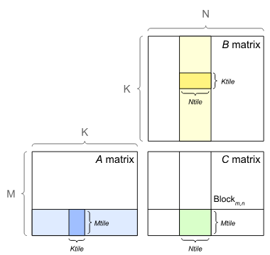
Figure 1. Tiled outer product approach to GEMMs

3.4. Tensor Core Requirements

As we discussed in GPU Architecture Fundamentals, the latest NVIDIA GPUs have introduced Tensor Cores to maximize the speed of tensor multiplies. Requirements to use Tensor Cores depend on NVIDIA library versions. Performance is better when equivalent matrix dimensions M M M, N N N, and K K K are aligned to multiples of 16 bytes (or 128 bytes on A100). With NVIDIA cuBLAS versions before 11.0 or NVIDIA cuDNN versions before 7.6.3, this is a requirement to use Tensor Cores; as of cuBLAS 11.0 and cuDNN 7.6.3, Tensor Cores may be used regardless, but efficiency is better when matrix dimensions are multiples of 16 bytes. For example, when using FP16 data, each FP16 element is represented by 2 bytes, so matrix dimensions would need to be multiples of 8 elements for best efficiency (or 64 elements on A100).

最新的NVIDIA GPU引入了Tensor Core，以最大限度地提高张量乘法的速度。使用Tensor Core的要求取决于NVIDIA库的版本。

Table 1. Tensor Core requirements by cuBLAS or cuDNN version for some common data precisions. These requirements apply to matrix dimensions M M M, N N N, and K K K.

Tensor Cores can be used for ...	cuBLAS version < 11.0, cuDNN version < 7.6.3	cuBLAS version ≥ 11.0, cuDNN version ≥ 7.6.3
INT8	Multiples of 16	Always but most efficient with multiples of 16; on A100, multiples of 128.
FP16	Multiples of 8	Always but most efficient with multiples of 8; on A100, multiples of 64.
TF32	N/A	Always but most efficient with multiples of 4; on A100, multiples of 32.
FP64	N/A	Always but most efficient with multiples of 2; on A100, multiples of 16.

The requirement is in fact more relaxed - only the fastest varying dimensions in memory are required to obey this rule - but it is easiest to just think of all three dimensions the same way.

实际上，这个要求比较宽松 - 只有内存中变化最快的维度才需要遵守这条规则 - 但最简单的办法就是把所有三个维度都看作是相同的。

Following these alignments for all dimensions ensures Tensor Cores will be enabled and run efficiently. This effect can be seen in Figure 5 - calculations are fastest (durations are lowest) when K is divisible by 8. When K K K is not divisible by 8, switching from cuBLAS 10.2 to cuBLAS 11.0 allows Tensor Cores to be used and results in 2-4x speedup. It is also worth noting that with cuBLAS 11.0, among values of K K K that are not divisible by 8, even values still result in faster calculation than odd values. We recommend choosing matrix dimensions to be multiples of 16 bytes (8 for FP16 as in Table 1); if this is not possible, choosing multiples of a smaller power of two (such as 8 or 4 bytes) often still helps performance with cuBLAS 11.0 and higher. On A100, choosing multiples of larger powers of two up to 128 bytes (64 for FP16) can further improve efficiency.

遵循这些维度对齐方式可确保启用 Tensor Core 并高效运行。如图 5 所示，当 K 能被 8 整除时，计算速度最快 (耗时最短)。当 K 不能被 8 整除时，从 cuBLAS 10.2 升级到 cuBLAS 11.0 可启用 Tensor Core，并带来 2-4 倍的加速。值得注意的是，在 cuBLAS 11.0 中，对于不能被 8 整除的 K 值，偶数仍然比奇数计算速度更快。我们建议矩阵维度选择为 16 字节的倍数 (如表 1 中 FP16 为 8 字节)；如果无法做到这一点，选择 2 的较小幂次方的倍数 (例如 8 或 4 字节) 通常仍然有助于提高 cuBLAS 11.0 及更高版本的性能。在 A100 上，选择 2 的较大幂次方，最大可达 128 字节 (FP16 为 64 字节)，可以进一步提高效率。

复制代码

1008 = 8 * 126
1012 = 4 * 253
1016 = 8 * 127
1020 = 4 * 255
1024 = 8 * 128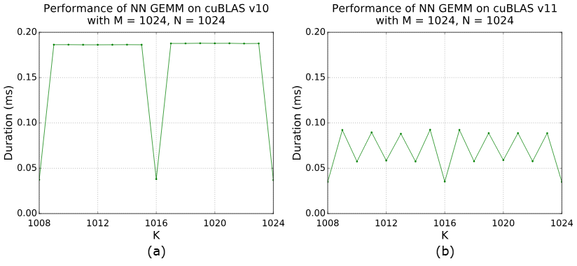

Figure 2. Comparison of GEMM execution times with (a) cuBLAS 10.1 and (b) cuBLAS 11.0, both with FP16 data. Calculation is fastest (duration is lowest) when K K K is divisible by 8. "NN" means A and B matrices are both accessed non-transposed. NVIDIA V100-DGXS-16GB GPU.

当 K 能被 8 整除时，计算速度最快 (耗时最短)。NN 表示矩阵 A 和 B 均以非转置形式访问。

3.5. Typical Tile Dimensions In cuBLAS And Performance

The cuBLAS library contains NVIDIA's optimized GPU GEMM implementations (refer to here for documentation).

While multiple tiling strategies are available, larger tiles have more data reuse, allowing them to use less bandwidth and be more efficient than smaller tiles.

虽然有多种分块策略可供选择，但较大的分块具有更高的数据复用率，因此比小分块占用更少的带宽，效率更高。

On the other hand, for a problem of a given size, using larger tiles will generate fewer tiles to run in parallel, which can potentially lead to under-utilization of the GPU.

另一方面，对于给定规模的问题，使用较大的分块会生成更少的并行运行分块，这可能会导致 GPU 利用率不足。

When frameworks like TensorFlow or PyTorch call into cuBLAS with specific GEMM dimensions, a heuristic inside cuBLAS is used to select one of the tiling options expected to perform the best. Alternatively, some frameworks provide a "benchmark" mode, where prior to the training they time all implementation choices and pick the fastest one (this constitutes a once per training session overhead).

当 TensorFlow 或 PyTorch 等框架使用特定的 GEMM 维度调用 cuBLAS 时，cuBLAS 内部会使用启发式算法来选择预期性能最佳的分块选项。此外，一些框架提供"基准测试"模式，在训练之前对所有实现方案进行计时，并选择速度最快的方案 (这会导致每次训练会话增加一次开销)。

This tradeoff between tile efficiency and tile parallelism suggests that the larger the GEMM, the less important this tradeoff is: at some point, a GEMM has enough work to use the largest available tiles and still fill the GPU. Conversely, if a GEMM is too small, the reduction in either tile efficiency or tile parallelism will likely prevent the GPU from running at peak math utilization. Figure 3 and Figure 4 illustrate this general trend; larger GEMMs achieve higher throughput.

这种分块效率和分块并行性之间的权衡表明，GEMM 越大，这种权衡就越不重要：在某个阶段，GEMM 的工作量足够大，可以使用最大的可用分块，并且仍然能够充分利用 GPU。相反，如果 GEMM 太小，分块效率或分块并行性的降低都可能导致 GPU 无法以最佳数学运算效率运行。图 3 和图 4 展示了这一总体趋势；更大的 GEMM 可以实现更高的吞吐量。

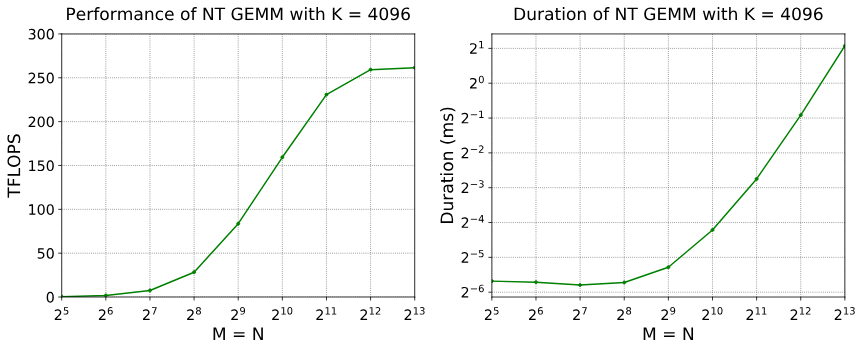
Figure 3. Performance improves as the M M M- N N N footprint of the GEMM increases. Duration also increases, but not as quickly as the M M M- N N N dimensions themselves; it is sometimes possible to increase the GEMM size (use more weights) for only a small increase in duration. NVIDIA A100-SXM4-80GB, CUDA 11.2, cuBLAS 11.4.

随着 GEMM 的 M M M- N N N 占用空间增大，性能得到提升。运行时间也会增加，但增长速度不如 M M M- N N N 维度本身的增长速度快；有时，增加 GEMM 的大小 (使用更多权重) 只会略微增加运行时间。

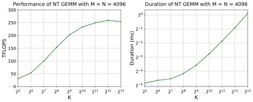
Figure 4. Performance improves as the K K K dimension increases, even when M = N M=N M=N is relatively large, as setup and tear-down overheads for the computation are amortized better when the dot product is longer. NVIDIA A100-SXM4-80GB, CUDA 11.2, cuBLAS 11.4.

随着 K K K 维数的增加，性能也会提高，即使 M = N M=N M=N 相对较大，因为当点积更长时，计算的设置和拆卸开销可以更好地摊销。

For cuBLAS GEMMs, thread block tile sizes typically but not necessarily use power-of-two dimensions.

对于 cuBLAS GEMM，线程块的瓦片大小通常 (但不一定) 使用 2 的幂次方。

Different tile sizes might be used for different use cases, but as a starting point, the following tiles are available:

256 × 128 256 \times 128 256×128 and 128 × 256 128 \times 256 128×256 (most efficient)
128 × 128 128 \times 128 128×128
256 × 64 256 \times 64 256×64 and 64 × 256 64 \times 256 64×256
128 × 64 128 \times 64 128×64 and 64 × 128 64 \times 128 64×128
64 × 64 64 \times 64 64×64 (least efficient)

Figure 5 shows an example of the efficiency difference between a few of these tile sizes.

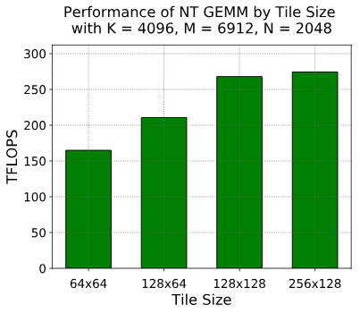
Figure 5. Larger tiles run more efficiently. The 256 × 128 256 \times 128 256×128-based GEMM runs exactly one tile per SM, the other GEMMs generate more tiles based on their respective tile sizes. NVIDIA A100-SXM4-80GB, CUDA 11.2, cuBLAS 11.4.

The chart shows the performance of a M × N × K = 6912 × 2048 × 4096 M \times N \times K = 6912 \times 2048 \times 4096 M×N×K=6912×2048×4096 GEMM with different tile sizes. It demonstrates that the increased tile parallelism with smaller tiles ( 64 × 64 64 \times 64 64×64 enables 8x more parallelism than 256 × 128 256 \times 128 256×128) comes at a notable efficiency cost. In practice, cuBLAS will avoid using small tiles for GEMMs that are large enough to have sufficient parallelism with larger tiles and will resort to the smaller ones only when substantially smaller GEMMs than the one in this example are being run. As a side note, NVIDIA libraries also have the ability to "tile" along the K K K dimension in case both M M M and N N N are small but K K K is large. Because K K K is the direction of the dot product, tiling in K K K requires a reduction at the end, which can limit achievable performance. For simplicity, most of this guide assumes no K K K tiling.

它表明，使用较小图块可以提高图块并行度，但会显著降低效率。实际上，cuBLAS 会避免对足够大的 GEMM 使用较小的图块，因为较大的图块就能提供足够的并行度；只有当运行的 GEMM 比本例中的 GEMM 小得多时，才会使用较小的图块。

4. Dimension Quantization Effects

As described in GPU Execution Model, a GPU function is executed by launching a number of thread blocks, each with the same number of threads. This introduces two potential effects on execution efficiency - tile and wave quantization.

GPU 函数的执行是通过启动若干线程块来实现的，每个线程块包含相同数量的线程。

4.1. Tile Quantization

Tile quantization occurs when matrix dimensions are not divisible by the thread block tile size.

The number of thread block tiles is large enough to make sure all output elements are covered, however, some tiles have very little actual work as illustrated in Figure 6, which assumes 128 × 128 128 \times 128 128×128 tiles and two matrix dimensions.

线程块图块的数量足够大，可以确保所有输出元素都被覆盖，但是，如图 6 所示，有些图块的实际工作量非常少，该图假设有 128 × 128 128 \times 128 128×128 个图块和两个矩阵维度。

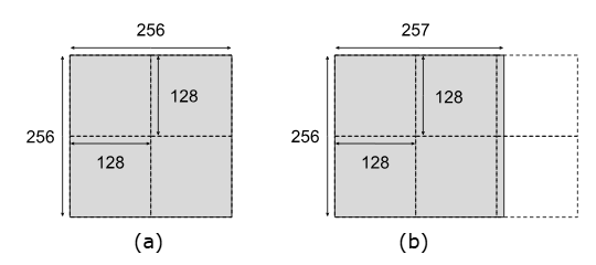
Figure 6. Example of tiling with 128 × 128 128 \times 128 128×128 thread block tiles. (a) Best case - matrix dimensions are divisible by tile dimensions (b) Worse case - tile quantization results in six thread blocks being launched, two of which waste most of their work.

While libraries ensure that invalid memory accesses are not performed by any of the tiles, all tiles will perform the same amount of math. Thus, due to tile quantization, the case in Figure 6 (b) executes 1.5x as many arithmetic operations as Figure 6 (a) despite needing only 0.39% more operations algorithmically. As this shows, the highest utilization is achieved when output matrix dimensions are divisible by tile dimensions.

尽管库确保所有图块都不会执行无效的内存访问，但所有图块执行的数学运算量相同。因此，由于图块量化，图 6 (b) 中的情况执行的算术运算次数是图 6 (a) 的 1.5 倍，尽管从算法角度来看，所需的运算次数仅增加了 0.39%。由此可见，当输出矩阵的维度能被图块的维度整除时，资源利用率最高。

For another example of this effect, let's consider GEMM for various choices of N N N, with M M M = 27648, K K K = 4096, and a library function that uses 256 × 128 256 \times 128 256×128 tile. As N N N increases from 136 to 256 in increments of 8, the Tensor Core accelerated GEMM always runs the same number of tiles, meaning the N N N dimension is always divided into 2 tiles. While the number of tiles remains constant, the fraction of those tiles containing useful data and hence the number of useful FLOPS performed an increase with N N N, as reflected by the GFLOPS in Figure 7 below. Notice that throughput reduces significantly between N N N = 128 (where the single tile per row is filled with useful data) and N N N = 136 (where a second tile is added per row but contains only 8/128 = 6.25% useful data). Also, note how the duration is constant whenever the number of tiles is constant.

为了进一步说明这种效应，我们考虑 GEMM 在不同 N N N 值下的性能，其中 M M M = 27648， K K K = 4096，并使用一个 256 × 128 256 \times 128 256×128 个 tile 的库函数。当 N N N 从 136 以 8 为增量增加到 256 时，Tensor Core 加速的 GEMM 始终运行相同数量的 tile，这意味着 N N N 维度始终被分成 2 个 tile。虽然 tile 的数量保持不变，但包含有用数据的 tile 比例 (因此有效 FLOPS 的数量) 随着 N N N 的增加而增加，如图 7 中的 GFLOPS 所示。请注意，吞吐量在 N N N = 128 (每行一个 tile 都填充了有用数据) 和 N N N = 136 (每行增加一个 tile，但仅包含 8/128 = 6.25% 的有用数据) 之间显著下降。另外，请注意，当图块数量恒定时，持续时间也是恒定的。

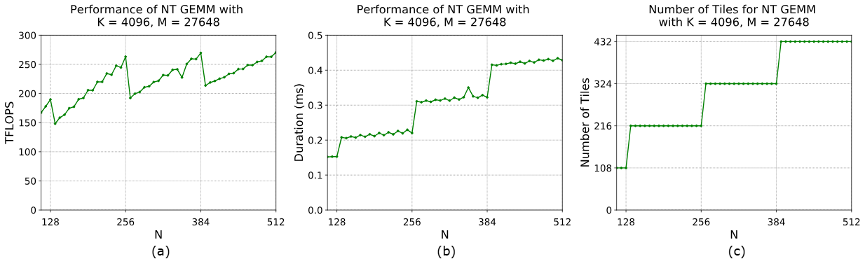
Figure 7. Tile quantization effect on (a) achieved FLOPS throughput and (b) elapsed time, alongside (c) the number of tiles created. Measured with a function that forces the use of 256 × 128 256 \times 128 256×128 tiles over the M × N M \times N M×N output matrix. In practice, cuBLAS would select narrower tiles (for example, 64-wide) to reduce the quantization effect. NVIDIA A100-SXM4-80GB, CUDA 11.2, cuBLAS 11.4.

4.2. Wave Quantization

While tile quantization means the problem size is quantized to the size of each tile, there is a second quantization effect where the total number of tiles is quantized to the number of multiprocessors on the GPU: Wave quantization.

Let's consider a related example to the one before, again varying N N N and with K K K = 4096, but with a smaller M M M = 2304. An NVIDIA A100 GPU has 108 SMs; in the particular case of 256 × 128 256 \times 128 256×128 thread block tiles, it can execute one thread block per SM, leading to a wave size of 108 tiles that can execute simultaneously. Thus, GPU utilization will be highest when the number of tiles is an integer multiple of 108 or just below.

NVIDIA A100 GPU 拥有 108 个 SM；在 256 × 128 个线程块的特定情况下，每个 SM 可以执行一个线程块，从而形成一个 108 个可以同时执行的线程块。因此，当线程块的数量是 108 的整数倍或略小于 108 时，GPU 利用率最高。

The M M M dimension will always be divided into 2304 / 256 = 9 tiles per column. When N N N = 1536, the N N N dimension is divided into 1536 / 128 = 12 tiles per row, and a total of 9 * 12 = 108 tiles are created, comprising one full wave. When 1536 < N N N <= 1664, an additional tile per row is created for a total of 9 * 13 = 117 tiles, leading to one full wave and a 'tail' wave of only 9 tiles. The tail wave takes nearly the same time to execute as the full 108-tile wave in this example but uses only 9 / 108 = 8.33% of A100's SMs during that time. Consequently, GFLOPS roughly halve and duration roughly doubles from N N N = 1536 to N N N = 1544 (Figure 8). Similar jumps can be seen after N N N = 3072, N N N = 4608, and N N N = 6144, which also map to an integer number of full waves.

M M M 维度始终每列被划分为 2304 / 256 = 9 个图块。当 N N N = 1536 时， N N N 维度每行被划分为 1536 / 128 = 12 个图块，总共生成 9 * 12 = 108 个图块，构成一个完整的 wave。当 1536 < N N N <= 1664 时，每行额外生成一个图块，总共生成 9 * 13 = 117 个图块，形成一个完整的 wave 和一个仅包含 9 个图块的 tail wave。在本例中，tail wave 的执行时间与完整的 108 个图块的 wave 几乎相同，但在此期间仅使用了 A100 的 9 / 108 = 8.33% 的 SM。因此，从 N N N = 1536 到 N N N = 1544，GFLOPS 大约减半，持续时间大约翻倍 (图 8)。在 N N N = 3072、 N N N = 4608 和 N N N = 6144 之后可以看到类似的跳跃，这也对应于整数个完整 waves。

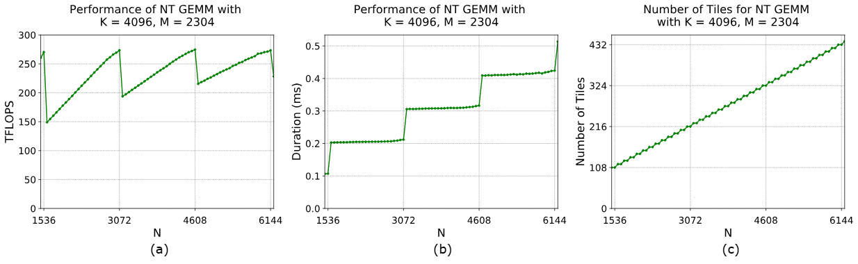
Figure 8. The effects of wave quantization in terms of (a) achieved FLOPS throughput and (b) elapsed time, as well as (c) the number of tiles created. Measured with a function that uses 256 × 128 256 \times 128 256×128 tiles over the M × N M \times N M×N output matrix. Note that the quantization effect occurs when the number of tiles passes a multiple of 108. NVIDIA A100-SXM4-80GB, CUDA 11.2, cuBLAS 11.4.

It is worth noting that the throughput and duration graphs for wave quantization look very similar to those for tile quantization, except with a different scale on the horizontal axis. Because both phenomena are quantization effects, this is expected. The difference lies in where the quantization occurs: tile quantization means work is quantized to the size of the tile, whereas wave quantization means work is quantized to the size of the GPU. Figure 7 (c) and Figure 8 (c) in both the tile and wave quantization illustrations show this difference.

References

$1$ Yongqiang Cheng (程永强), https://yongqiang.blog.csdn.net/

$2$ Matrix Multiplication Background User's Guide, https://docs.nvidia.com/deeplearning/performance/dl-performance-matrix-multiplication/index.html

$3$ Matrix Multiplication Performance (矩阵乘法性能), https://mp.weixin.qq.com/s/YaQG5RR6qbEZXX0ehbMHAg