Vladimir Arnold(算是前苏联神通)和其导师Andrey Kolmogorov(前苏联科学院院士)证明
如果是有界域上的多元连续函数(if f is a multivariate continuous function
on a bounded domain ),则可以写成有限个连续函数 的复合单变量和加法的二元运算(then f can be written as a finite composition of continuous functions of**a single variable and the binary operation of addition)
总之,每个函数都可以用一元函数 和求和 来表示(since every other function can be written using univariate functions and sum),看似前途一片光明,因为学习高维函数可以因此归结为学习多项式数量的一维函数(learning a high-dimensional function boils down to learning a polynomial number of 1D functions)
然而,这些一维函数可能是非光滑甚至是分形的,因此在实践中可能无法学习(However, these 1D functions can be non-smooth and even fractal, so they may not be learnable in practice)
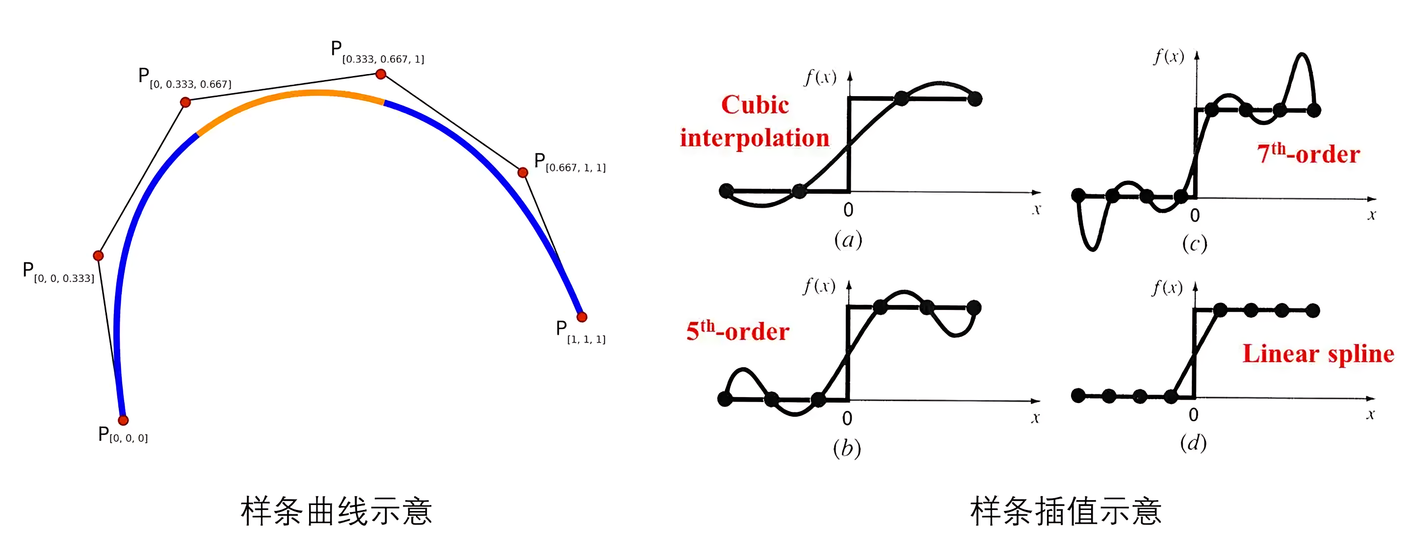
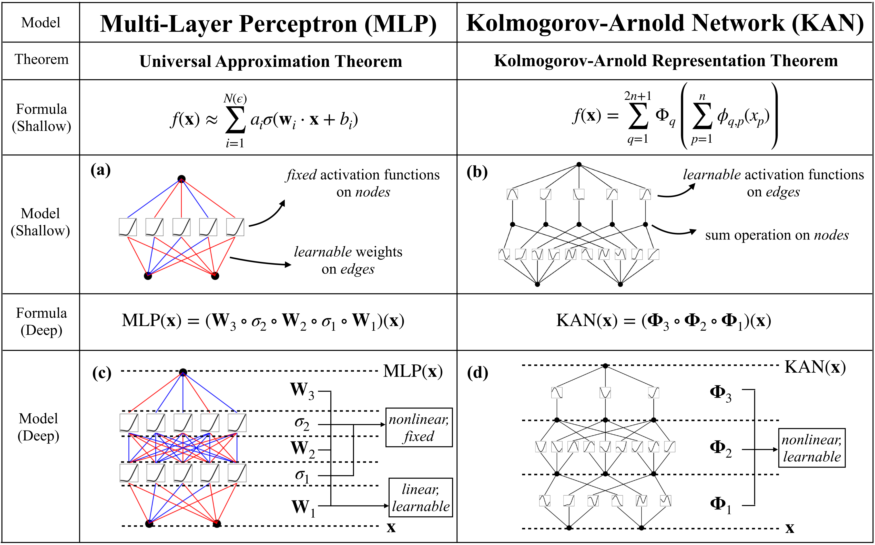
splines 在低维函数中是准确的,易于局部调整,并能够在不同分辨率之间切换。 然而,splines存在严重的维度问题,无法利用组合结构 (splines have a serious curse of dimensionality (COD) problem, because of their inability to exploit compositional structures)
另一方面,MLP 相对于维度问题的影响较小(归功于它们的特征学习),但在低维度下比splines不够准确,无法优化单变量函数 (because of their inability to optimize univariate function)
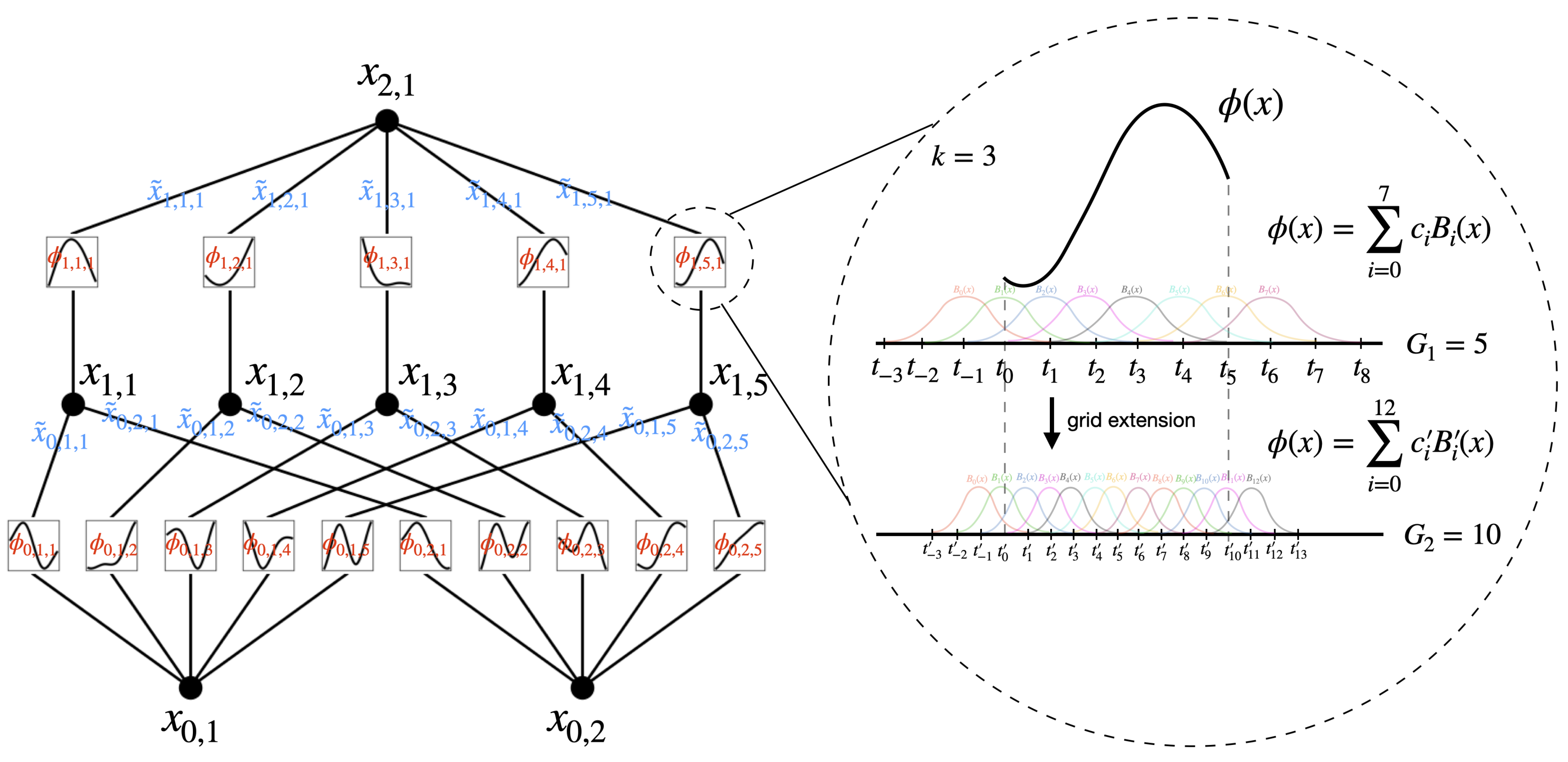
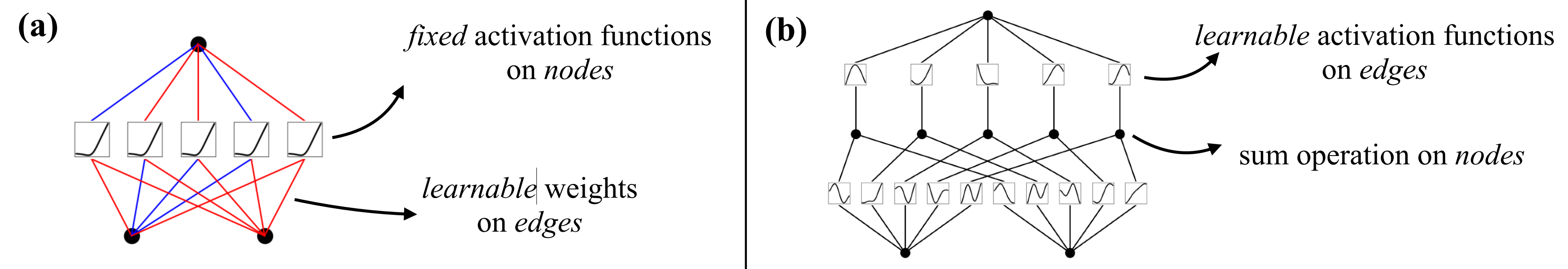
由于KANs
在内部有splines「splines有内部自由度,但没有外部自由度,即splines有内无外,至于所谓自由度,指的是The computational graph of hown odes are connected represents external degrees of freedom (即节点之间的连接代表自由度:"dofs")」
还可以将这些学到的特征优化到极高的准确度(与样条的内部相似性),即可以很好地近似单变量函数(即learning univariate functions)
且在外部有MLPs(MLPs有外部自由度,但没内部自由度,MLPs有外无内)
因此,KANs不仅可以学习特征(与MLPs的外部相似性),即可以学习多个变量的组合结构(learning compositional structures of multiple variables)
初始化规模
每个激活函数的初始化值为(这是通过绘制 B 样条系数 ci∼ N (0, σ2)来完成的,其中σ很小,通常我们设置σ= 0.1) 则根据Xavier初始化进行初始化(该初始化方法已用于初始化MLP中的线性层)
Update of spline grids
根据其输入激活实时更新每个格网,以解决splines在有界区域上定义,但激活值在训练过程中可能超出固定区域的问题(We update each grid on the fly according to its input activations, to address the issue that splines are defined on bounded regions but activation values can evolve out of the fixed region during training)
我们考虑允许表示成任意宽和深,以具备激活平滑性,如方程2.7中所示「To facilitate an approximation analysis, we still assume smoothness of activations, but allow the representations to be arbitrarily wide and deep, as in Eq. (2.7)」
那么存在一个取决于 和其表示的常数,使得有以下关于网格大小 的逼近界限: 存在k-th order B-spline函数,对于任意 ,有界限 (*such that we have the following approximation bound in terms of thegrid size G: there exist k-th order B-spline functions ΦGl,i,jsuch that for any 0 ≤ m ≤ k, we have the bound,*以下公式定义为2.15)
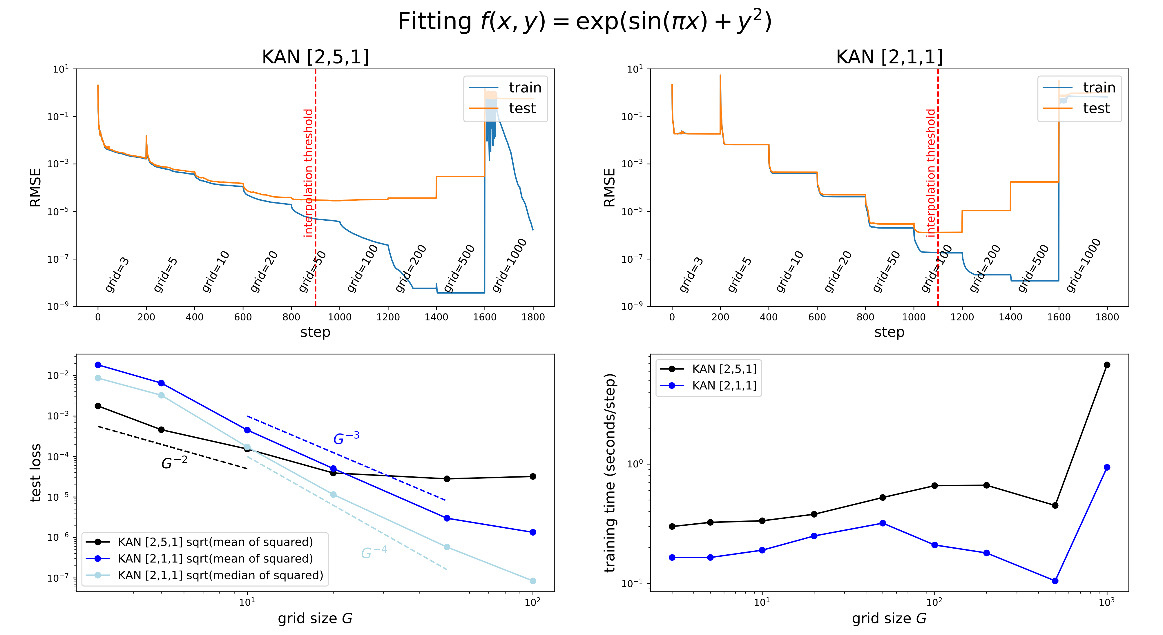
如上图左上角所示,展示了一个 2, 5, 1KAN的训练和测试RMSE
网格点的数量从3开始,每200个LBFGS步骤增加到更高的值,最终达到1000个网格点
很明显,每次进行精细化处理时,训练损失下降速度比以前快(除了具有1000个点的最细网格,由于糟糕的loss landscapes,优化停止工作)
然而,测试损失先下降然后上升,显示出U形状,这是由于偏差-方差权衡(欠拟合与过拟合)造成的
作者推测,当参数数量与数据点数量匹配时,最佳测试损失是在插值阈值 处实现的(We conjecture that the optimal test loss is achieved at the interpolation thresholdwhen the number of parameters match the number of data points)
比如由于训练样本有1000个,而一个2, 5, 1KAN的总参数为 (G是网格间隔的数量),作者预计插值阈值为G= 1000/15 ≈ 67,这与作者实验观察到的值 G ∼ 50大致吻合
如上图左下角所示 ,随着网格数量的增加:比如从、到,测试的损失也会随之而降低
且可以看到(为方便大家把图和文字一一对应,所以下面在描述不同的曲线时,我特意用了不同的颜色 ) 一个2,1,1 KAN的测试RMSE大致按照测试RMSE ∝ 的比例变化(a 2,1,1 KAN scales roughly as test RMSE ∝ G−3) 且当绘制平方根的中位数(而不是均值)的平方损失时,2,1,1 KAN的测试RMSE则更接近 的缩放(If we plot the square root of the median (not mean) of the squared losses, we get a scaling closer to G−4. 其实这样才正常,毕竟according to the Theorem 2.1, we would expect test RMSE ∝ G−4 )
最后,如上图右下角所示 ,训练时间随着网格点数 G的增加而有利
比如无论是2,5,1 KAN,还是2,1,1 KAN,在后半段(除了最后一小节)都有一段随着网格点数增加而训练时间减少的走势,特别是后者2,1,1 KAN
稀疏化Sparsification (相当于预处理)
对于MLP,使用线性权重的L1正则化来偏好稀疏性(L1 regularization of linear weights is used to favor sparsity)
KAN可以采纳MLP这个思路,但需要两个修改:
(1) KAN中没有线性"权重",因为线性权重被可学习的激活函数取代了,因此需要定义这些激活函数的L1范数
(2) 但L1对于KAN的稀疏化是不够的,所以还需要额外的熵正则化
可视化Visualization
当可视化一个KAN时,为了感受到幅度,将激活函数的透明度设
置成的比例,其中 β= 3。 因此,具有较小幅度的函数会被忽略,好聚焦于重要函数(When we visualize a KAN, to get a sense of magnitudes, we set the transparency of an activation function ϕl,i,j proportional to tanh(βAl,i,j ) where β = 3 . Hence, functions with small magnitude appear faded out to allow us to focus on important ones)
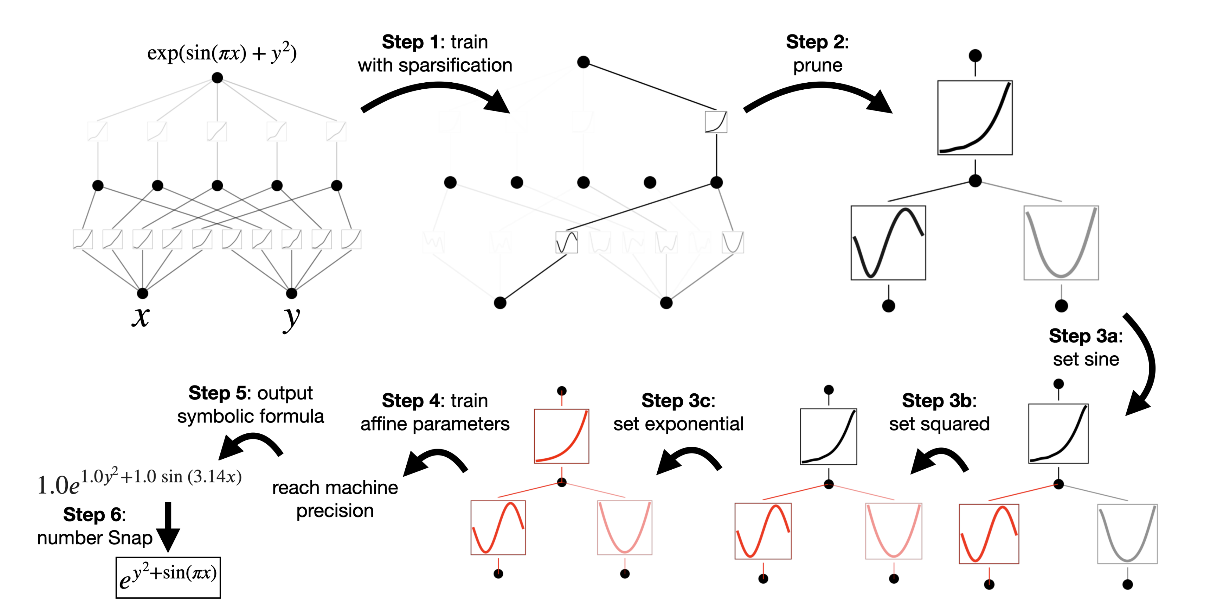
Symbolification
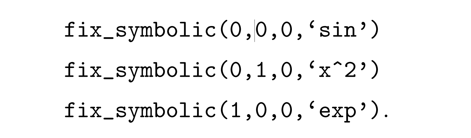
在我们怀疑某些激活函数实际上是符号化的情况下(例如cos或 log),提供一个接口来将它们设置为指定的符号形式(*we provide an interface to set them to be a specified symbolic f),*fix_symbolic(l,i,j,f) 可以将激活设置为
然而,不能简单地将激活函数设置为精确的符号公式,因为它的输入和输出可能存在偏移和缩放
因此,从样本中获得预激活 x和后激活 y(we obtain preactivations x and postactivations y from samples),并拟合仿射参数使得(这里的拟合可通过迭代网格搜索a, b 和线性回归来完成)
是有界域上的多元连续函数(if f is a multivariate continuous function