1 导入必要的库
python
import pandas as pd
import numpy as np
import matplotlib.pyplot as plt
from sklearn.model_selection import train_test_split
from sklearn.preprocessing import LabelEncoder
from tensorflow.keras.models import Sequential
from tensorflow.keras.layers import Dense
from tensorflow.keras.callbacks import EarlyStopping
from sklearn.metrics import classification_report, confusion_matrix
# 忽略Matplotlib的警告(可选)
import warnings
warnings.filterwarnings("ignore")
# 设置中文显示和负号正常显示
plt.rcParams['font.sans-serif'] = ['SimHei']
plt.rcParams['axes.unicode_minus'] = False
2 数据加载与预处理
python
# 读取数据
df = pd.read_csv('train.csv')

# 处理缺失值(这里假设我们删除含有缺失值的行)
df.dropna(inplace=True)

# 处理重复值(这里选择删除重复的行)
df.drop_duplicates(inplace=True)

# 将'wine types'列的文本转换为数值
df['wine types'] = df['wine types'].map({'red': 1, 'white': 2})
# 假设'quality'是我们要预测的标签
X = df.drop('quality', axis=1)
y = df['quality']
3 数据探索
python
# 选择绘制特征数据的折线图
X_columns_to_plot = X.columns

df_plot = df[X_columns_to_plot]

df_plot.plot(subplots=True, figsize=(15, 15))
plt.tight_layout()
plt.show()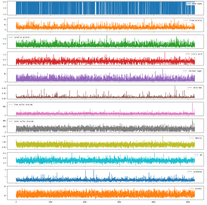
图 3-1
4 BP神经网络模型构建
python
import tensorflow as tf
from tensorflow.keras.models import Sequential
from tensorflow.keras.layers import Dense
from sklearn.model_selection import train_test_split
from sklearn.preprocessing import StandardScaler

# 分离特征和标签
X = df.drop('quality', axis=1)
y = df['quality']

# 划分训练集和测试集
X_train, X_test, y_train, y_test = train_test_split(X, y, test_size=0.2, random_state=42)

# 特征缩放
scaler = StandardScaler()
X_train_scaled = scaler.fit_transform(X_train)
X_test_scaled = scaler.transform(X_test)

# 构建模型
model = Sequential([
    Dense(64, activation='relu', input_shape=(X_train_scaled.shape[1],)),
    Dense(32, activation='relu'),
    Dense(10, activation='softmax')  # 假设有10个类别,根据实际情况调整
])

# 编译模型
model.compile(optimizer='adam', loss='sparse_categorical_crossentropy', metrics=['accuracy'])

# 训练模型
history = model.fit(X_train_scaled, y_train, epochs=100, validation_split=0.2, verbose=1)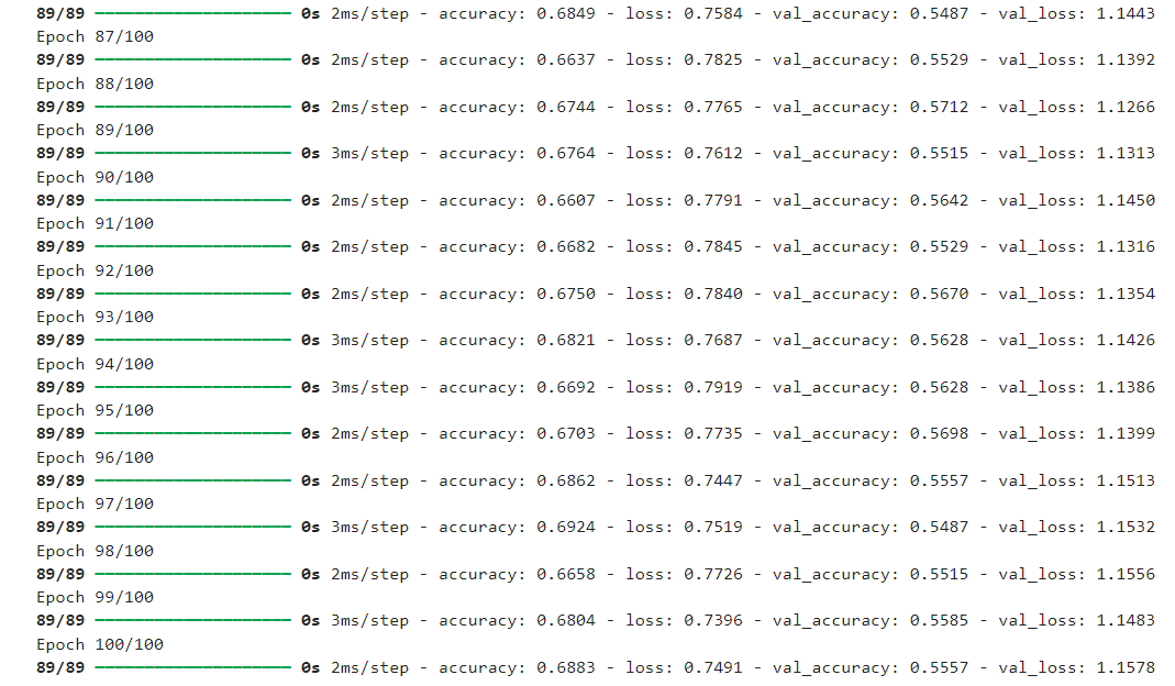
图 4-1
5 训练评估可视化
python
# 绘制训练和验证的准确率与损失
plt.figure(figsize=(12, 6))
plt.subplot(1, 2, 1)
plt.plot(history.history['accuracy'], color='#B0D5DF',label='Training Accuracy')
plt.plot(history.history['val_accuracy'],  color='#1BA784',label='Validation Accuracy')
plt.title('Training and Validation Accuracy')
plt.legend()

plt.subplot(1, 2, 2)
plt.plot(history.history['loss'],  color='#D11A2D',label='Training Loss')
plt.plot(history.history['val_loss'], color='#87723E', label='Validation Loss')
plt.title('Training and Validation Loss')
plt.legend()
plt.show()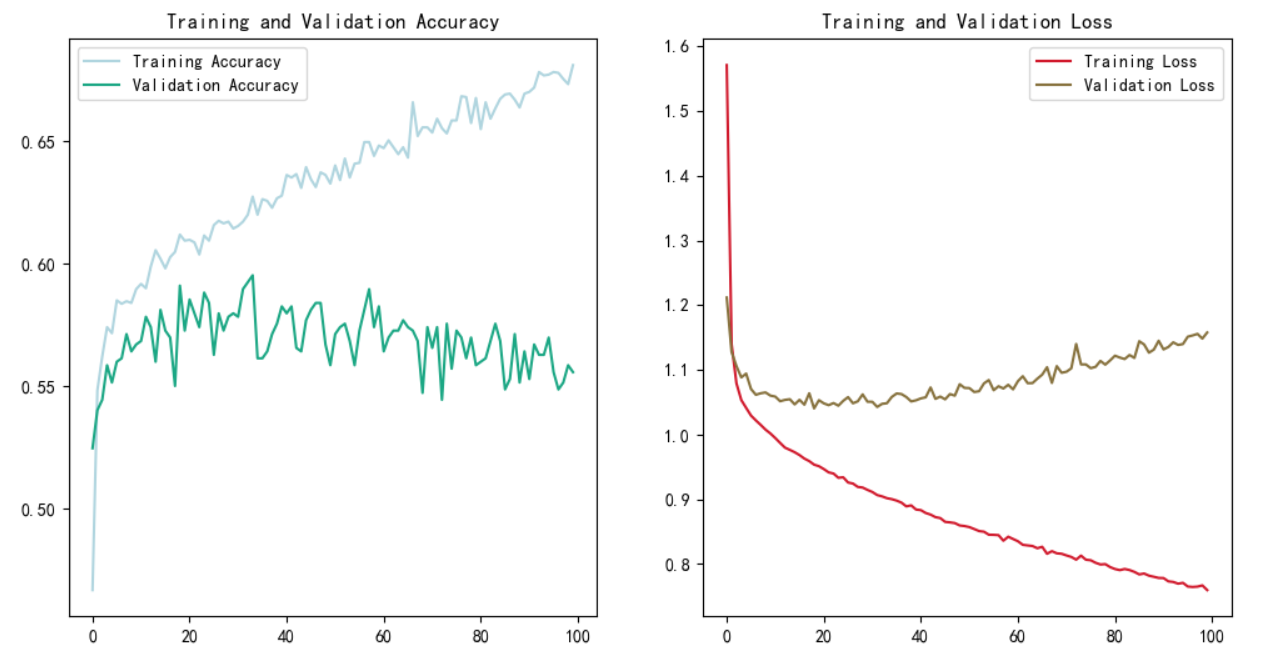
图 5-1 过拟合
成功过拟合了,其实早有预料,我手里的数据集都挺顽固的,训练效果都不好。
6 正则化
这里采用L2正则化
python
import tensorflow as tf
from tensorflow.keras.models import Sequential
from tensorflow.keras.layers import Dense
from tensorflow.keras.regularizers import l2
from sklearn.model_selection import train_test_split
from sklearn.preprocessing import StandardScaler

# 分离特征和标签
X = df.drop('quality', axis=1)
y = df['quality']

# 划分训练集和测试集
X_train, X_test, y_train, y_test = train_test_split(X, y, test_size=0.2, random_state=42)

# 特征缩放
scaler = StandardScaler()
X_train_scaled = scaler.fit_transform(X_train)
X_test_scaled = scaler.transform(X_test)

# 构建模型,添加L2正则化
model = Sequential([
    Dense(64, activation='relu', input_shape=(X_train_scaled.shape[1],), kernel_regularizer=l2(0.01)),  # 对第一个Dense层的权重添加L2正则化
    Dense(64, activation='relu', kernel_regularizer=l2(0.01)),  # 对第二个Dense层的权重也添加L2正则化
    Dense(10, activation='softmax')  # 输出层,假设是多分类问题
])

# 编译模型
model.compile(optimizer='adam', loss='sparse_categorical_crossentropy', metrics=['accuracy'])

# 训练模型
history = model.fit(X_train_scaled, y_train, epochs=100, validation_split=0.2, verbose=1)
python
# 绘制训练和验证的准确率与损失
plt.figure(figsize=(12, 6))
plt.subplot(1, 2, 1)
plt.plot(history.history['accuracy'], color='#B0D5DF',label='Training Accuracy')
plt.plot(history.history['val_accuracy'],  color='#1BA784',label='Validation Accuracy')
plt.title('Training and Validation Accuracy')
plt.legend()

plt.subplot(1, 2, 2)
plt.plot(history.history['loss'],  color='#D11A2D',label='Training Loss')
plt.plot(history.history['val_loss'], color='#87723E', label='Validation Loss')
plt.title('Training and Validation Loss')
plt.legend()
plt.show()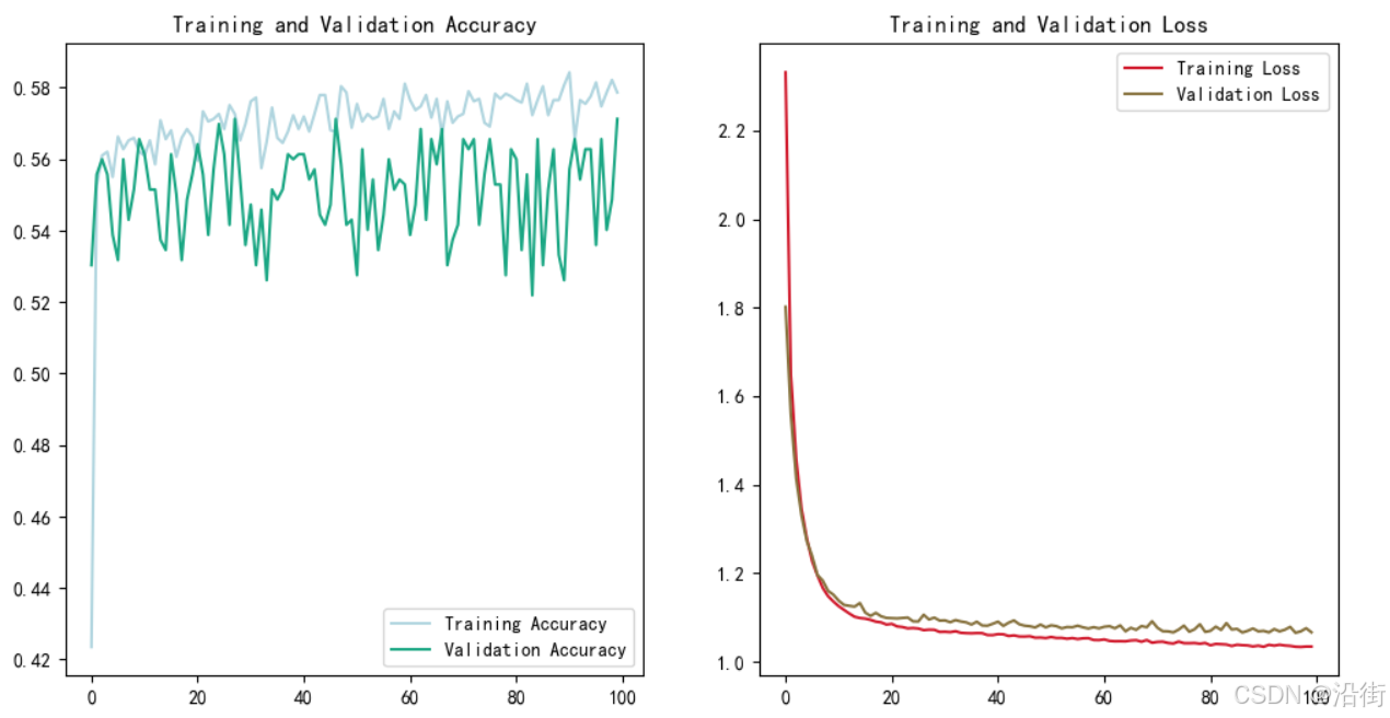
图 6-1
这就不错了。