002 | 常见的金融量化指标计算

金融量化指标

在金融量化分析中，常用的指标可以帮助我们判断市场走势、评估风险和收益，以及构建交易策略。以下是一些常见的金融量化指标及其计算方法的详细教程，包括公式与Python代码实现。

1. 移动平均线（Moving Average, MA）

简介：移动平均线是对特定时期内的数据进行平均，以平滑价格波动，从而帮助识别趋势方向。

公式：
M A n = P 1 + P 2 + . . . + P n n MA_n = \frac{P_1 + P_2 + ... + P_n}{n} MAn=nP1+P2+...+Pn

其中， P i P_i Pi 是第 i i i天的收盘价， n n n 是移动平均的周期。

Python代码：

python 复制代码

import pandas as pd

def moving_average(prices, window):
    return prices.rolling(window=window).mean()

# 示例
data = pd.Series([100, 102, 101, 104, 106, 108])
ma = moving_average(data, 3)
print(ma)

2. 指数平滑移动平均线（Exponential Moving Average, EMA）

简介：EMA对最近的数据赋予更大的权重，从而比简单移动平均线更快地响应价格变化。

公式：
E M A t = α × P t + ( 1 − α ) × E M A t − 1 EMA_t = \alpha \times P_t + (1 - \alpha) \times EMA_{t-1} EMAt=α×Pt+(1−α)×EMAt−1

其中， α = 2 n + 1 \alpha = \frac{2}{n+1} α=n+12， n n n 是平滑周期。

Python代码：

python 复制代码

def exponential_moving_average(prices, window):
    return prices.ewm(span=window, adjust=False).mean()

# 示例
ema = exponential_moving_average(data, 3)
print(ema)

3. 相对强弱指数（Relative Strength Index, RSI）

简介：RSI衡量股票价格的上涨和下跌的速度，用于判断市场是否超买或超卖。

公式：
R S I = 100 − 100 1 + R S RSI = 100 - \frac{100}{1 + RS} RSI=100−1+RS100

其中，(RS = \frac{\text{平均上涨值}}{\text{平均下跌值}})。

Python代码：

python 复制代码

def relative_strength_index(prices, window=14):
    delta = prices.diff()
    gain = (delta.where(delta > 0, 0)).rolling(window=window).mean()
    loss = (-delta.where(delta < 0, 0)).rolling(window=window).mean()
    rs = gain / loss
    rsi = 100 - (100 / (1 + rs))
    return rsi

# 示例
rsi = relative_strength_index(data, 14)
print(rsi)

4. 移动平均收敛散度（Moving Average Convergence Divergence, MACD）

简介：MACD是两条指数移动平均线之间的差值，用于判断价格走势的变化趋势。

公式：
M A C D = E M A 12 − E M A 26 MACD = EMA_{12} - EMA_{26} MACD=EMA12−EMA26
S i g n a l = E M A 9 ( M A C D ) Signal = EMA_{9}(MACD) Signal=EMA9(MACD)

Python代码：

python 复制代码

def macd(prices, short_window=12, long_window=26, signal_window=9):
    ema_short = exponential_moving_average(prices, short_window)
    ema_long = exponential_moving_average(prices, long_window)
    macd_line = ema_short - ema_long
    signal_line = exponential_moving_average(macd_line, signal_window)
    return macd_line, signal_line

# 示例
macd_line, signal_line = macd(data)
print(macd_line, signal_line)

5. 布林带（Bollinger Bands）

简介：布林带由三条线组成，中间的线是移动平均线，上下两条线分别是移动平均线加减一定倍数的标准差，用于衡量价格的波动范围。

公式：
上轨 = M A + k × σ \text{上轨} = MA + k \times \sigma 上轨=MA+k×σ
下轨 = M A − k × σ \text{下轨} = MA - k \times \sigma 下轨=MA−k×σ

其中， M A MA MA 是移动平均线， σ \sigma σ 是价格的标准差， k k k 是调整因子，一般取2。

Python代码：

python 复制代码

def bollinger_bands(prices, window=20, num_std_dev=2):
    ma = moving_average(prices, window)
    std_dev = prices.rolling(window=window).std()
    upper_band = ma + num_std_dev * std_dev
    lower_band = ma - num_std_dev * std_dev
    return upper_band, lower_band

# 示例
upper_band, lower_band = bollinger_bands(data)
print(upper_band, lower_band)

6. 平均真实波动范围（Average True Range, ATR）

简介：ATR用于衡量市场的波动性，反映了价格波动的剧烈程度。

公式：
T R = max ⁡ ( 当前最高价 − 当前最低价 , ∣ 当前最高价 − 前一收盘价 ∣ , ∣ 当前最低价 − 前一收盘价 ∣ ) TR = \max(\text{当前最高价} - \text{当前最低价}, |\text{当前最高价} - \text{前一收盘价}|, |\text{当前最低价} - \text{前一收盘价}|) TR=max(当前最高价−当前最低价,∣当前最高价−前一收盘价∣,∣当前最低价−前一收盘价∣)
A T R = ∑ i = 1 n T R i n ATR = \frac{\sum_{i=1}^{n} TR_i}{n} ATR=n∑i=1nTRi

Python代码：

python 复制代码

def true_range(high, low, close):
    return pd.concat([high - low, 
                      (high - close.shift()).abs(), 
                      (low - close.shift()).abs()], axis=1).max(axis=1)

def average_true_range(high, low, close, window=14):
    tr = true_range(high, low, close)
    atr = tr.rolling(window=window).mean()
    return atr

# 示例
high = pd.Series([105, 107, 110, 112])
low = pd.Series([100, 102, 104, 109])
close = pd.Series([102, 106, 108, 111])
atr = average_true_range(high, low, close)
print(atr)

7. 威廉指标（Williams %R）

简介：威廉指标用于判断市场的超买或超卖状态，数值范围在-100到0之间。

公式：
% R = 最高价 n − 收盘价最高价 n − 最低价 n × ( − 100 ) \%R = \frac{\text{最高价}_n - \text{收盘价}}{\text{最高价}_n - \text{最低价}_n} \times (-100) %R=最高价n−最低价n最高价n−收盘价×(−100)

其中，最高价 n \text{最高价}_n 最高价n 和最低价 n \text{最低价}_n 最低价n 分别为过去n天内的最高和最低价格。

Python代码：

python 复制代码

def williams_r(high, low, close, window=14):
    highest_high = high.rolling(window=window).max()
    lowest_low = low.rolling(window=window).min()
    wr = (highest_high - close) / (highest_high - lowest_low) * -100
    return wr

# 示例
wr = williams_r(high, low, close)
print(wr)

8. 随机指标（Stochastic Oscillator）

简介：随机指标用于衡量收盘价在最近一段时间价格范围内的位置，判断价格的超买或超卖情况。

公式：
K = 收盘价 − 最低价 n 最高价 n − 最低价 n × 100 K = \frac{\text{收盘价} - \text{最低价}_n}{\text{最高价}_n - \text{最低价}_n} \times 100 K=最高价n−最低价n收盘价−最低价n×100
D = ∑ K 3 D = \frac{\sum K}{3} D=3∑K

Python代码：

python 复制代码

def stochastic_oscillator(high, low, close, window=14):
    lowest_low = low.rolling(window=window).min()
    highest_high = high.rolling(window=window).max()
    k = (close - lowest_low) / (highest_high - lowest_low) * 100
    d = k.rolling(window=3).mean()
    return k, d

# 示例
k, d = stochastic_oscillator(high, low, close)
print(k, d)

9. 平滑异同平均指标（Smoothed Moving Average, SMA）

简介：SMA是将移动平均和当前价格进行平滑处理的指标，比EMA更加平滑。

公式：
S M A t = ∑ i = 1 n P i n SMA_t = \frac{\sum_{i=1}^{n} P_i}{n} SMAt=n∑i=1nPi

其中， P i P_i Pi 是价格数据， n n n 是时间周期。

Python代码：

python 复制代码

def smoothed_moving_average(prices, window):
    return prices.rolling(window=window).mean()

# 示例
sma = smoothed_moving_average(data, 3)
print(sma)

10. 波动率（Volatility）

简介：波动率是衡量价格变化的剧烈程度的重要指标，通常用标准差表示。

公式：
Volatility = ∑ i = 1 n ( P i − M A ) 2 n \text{Volatility} = \sqrt{\frac{\sum_{i=1}^{n} (P_i - MA)^2}{n}} Volatility=n∑i=1n(Pi−MA)2

Python代码：

python 复制代码

def volatility(prices, window):
    return prices.rolling(window=window).std()

# 示例
vol = volatility(data, 10)
print(vol)

11. 商品通道指数（Commodity Channel Index, CCI）

简介：CCI衡量价格相对于其均值的偏离程度，用于判断市场的超买或超卖状态。

公式：
C C I = P t − M A t 0.015 × M D CCI = \frac{P_t - MA_t}{0.015 \times MD} CCI=0.015×MDPt−MAt

其中，(P_t) 是典型价格，(MA_t) 是移动平均，(MD) 是均方差。

Python代码：

python 复制代码

def commodity_channel_index(high, low, close, window=20):
    tp = (high + low + close) / 3
    ma = tp.rolling(window=window).mean()
    md = tp.rolling(window=window).apply(lambda x: pd.Series(x).mad())
    cci = (tp - ma) / (0.015 * md)
    return cci

# 示例
cci = commodity_channel_index(high, low, close)
print(cci)

12. 恐慌指数（VIX）

简介：VIX是衡量市场对未来30天价格波动预期的指标，通常被称为"恐慌指数"。

公式：VIX的计算比较复杂，通常基于标普500指数期权的隐含波动率来计算。它的公式涉及多个期权的计算，这里简化为波动率的代表。

Python代码：

python 复制代码

import numpy as np

def vix(prices):
    log_returns = np.log(prices / prices.shift(1))
    vol = log_returns.rolling(window=30).std() * np.sqrt(252)
    return vol

# 示例
vix_index = vix(data)
print(vix_index)

13. 收益率（Rate of Return, RoR）

简介：收益率是衡量投资或资产在特定时间内的增长或减少百分比。它通常用来评估投资的盈利能力。

公式：

简单收益率 ：
Simple Return = P t − P t − 1 P t − 1 × 100 % \text{Simple Return} = \frac{P_t - P_{t-1}}{P_{t-1}} \times 100\% Simple Return=Pt−1Pt−Pt−1×100%

其中，(P_t) 是当前价格，(P_{t-1}) 是前一时间点的价格。
对数收益率 ：
Log Return = ln ⁡ ( P t P t − 1 ) \text{Log Return} = \ln\left(\frac{P_t}{P_{t-1}}\right) Log Return=ln(Pt−1Pt)

Python代码：

python 复制代码

import numpy as np

def simple_return(prices):
    return (prices / prices.shift(1)) - 1

def log_return(prices):
    return np.log(prices / prices.shift(1))

# 示例
simple_r = simple_return(data)
log_r = log_return(data)
print(simple_r, log_r)

使用 Tushare 计算所有指标的综合示例

Tushare 是一个用于获取中国市场数据的开源Python包。我们将使用 Tushare 下载股票数据并计算上面介绍的指标。

1. 安装 Tushare

如果你还没有安装 Tushare，可以使用以下命令进行安装：

bash 复制代码

pip install tushare

2. 获取股票数据

首先，我们需要获取股票的历史价格数据。

python 复制代码

import tushare as ts
import pandas as pd

# 设置你的 Tushare token
ts.set_token('your_token_here')
pro = ts.pro_api()

# 获取某只股票的日线数据
data = pro.daily(ts_code='000001.SZ', start_date='20220101', end_date='20221231')

# 将数据按日期排序并设置日期为索引
data['trade_date'] = pd.to_datetime(data['trade_date'])
data = data.sort_values(by='trade_date')
data.set_index('trade_date', inplace=True)

# 提取收盘价、高低价等数据
close = data['close']
high = data['high']
low = data['low']

3. 计算所有指标

我们将结合之前编写的函数，计算所有的指标：

python 复制代码

# 移动平均线
ma_20 = moving_average(close, 20)

# 指数平滑移动平均线
ema_20 = exponential_moving_average(close, 20)

# 相对强弱指数
rsi_14 = relative_strength_index(close, 14)

# 移动平均收敛散度
macd_line, signal_line = macd(close)

# 布林带
upper_band, lower_band = bollinger_bands(close)

# 平均真实波动范围
atr_14 = average_true_range(high, low, close, 14)

# 威廉指标
wr_14 = williams_r(high, low, close, 14)

# 随机指标
k, d = stochastic_oscillator(high, low, close, 14)

# 平滑异同平均指标
sma_20 = smoothed_moving_average(close, 20)

# 波动率
vol_10 = volatility(close, 10)

# 商品通道指数
cci_20 = commodity_channel_index(high, low, close, 20)

# 恐慌指数（这里使用对数收益率的波动率表示）
vix_index = vix(close)

# 简单收益率
simple_r = simple_return(close)

# 对数收益率
log_r = log_return(close)

4. 将所有指标汇总为一个 DataFrame

python 复制代码

# 将所有计算的指标放入一个 DataFrame 中
indicators = pd.DataFrame({
    'MA_20': ma_20,
    'EMA_20': ema_20,
    'RSI_14': rsi_14,
    'MACD_Line': macd_line,
    'Signal_Line': signal_line,
    'Upper_Band': upper_band,
    'Lower_Band': lower_band,
    'ATR_14': atr_14,
    'WR_14': wr_14,
    'K': k,
    'D': d,
    'SMA_20': sma_20,
    'Volatility_10': vol_10,
    'CCI_20': cci_20,
    'VIX_Index': vix_index,
    'Simple_Return': simple_r,
    'Log_Return': log_r
})

print(indicators.head())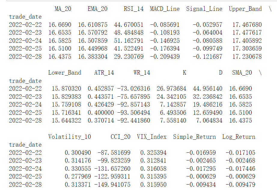

总结

通过上述代码，我们展示了如何使用 Tushare 获取股票数据，并计算多种常见的金融量化指标。这些指标可以帮助分析市场趋势、评估风险和收益，从而构建更为复杂的交易策略。在实际应用中，可以根据自己的需求调整指标的参数和选择的时间窗口，并结合其他数据源和工具进行更深入的分析。