Tensorflow2实现: LSTM-火灾温度预测

**🍨 本文为[🔗365天深度学习训练营](https://mp.weixin.qq.com/s/rnFa-IeY93EpjVu0yzzjkw) 中的学习记录博客**
**🍖 原作者：[K同学啊](https://mtyjkh.blog.csdn.net/)**

一：理论知识基础

1.LSTM原理

一句话介绍LSTM，它是RNN的进阶版, 如果说RNN的最大限度是理解一句话，那么LSTM的最大限度则是理解一段话，详细介绍如下：

LSTM，全称为长短记忆网络，是一种特殊的RNN，能够学习到长期依赖关系。

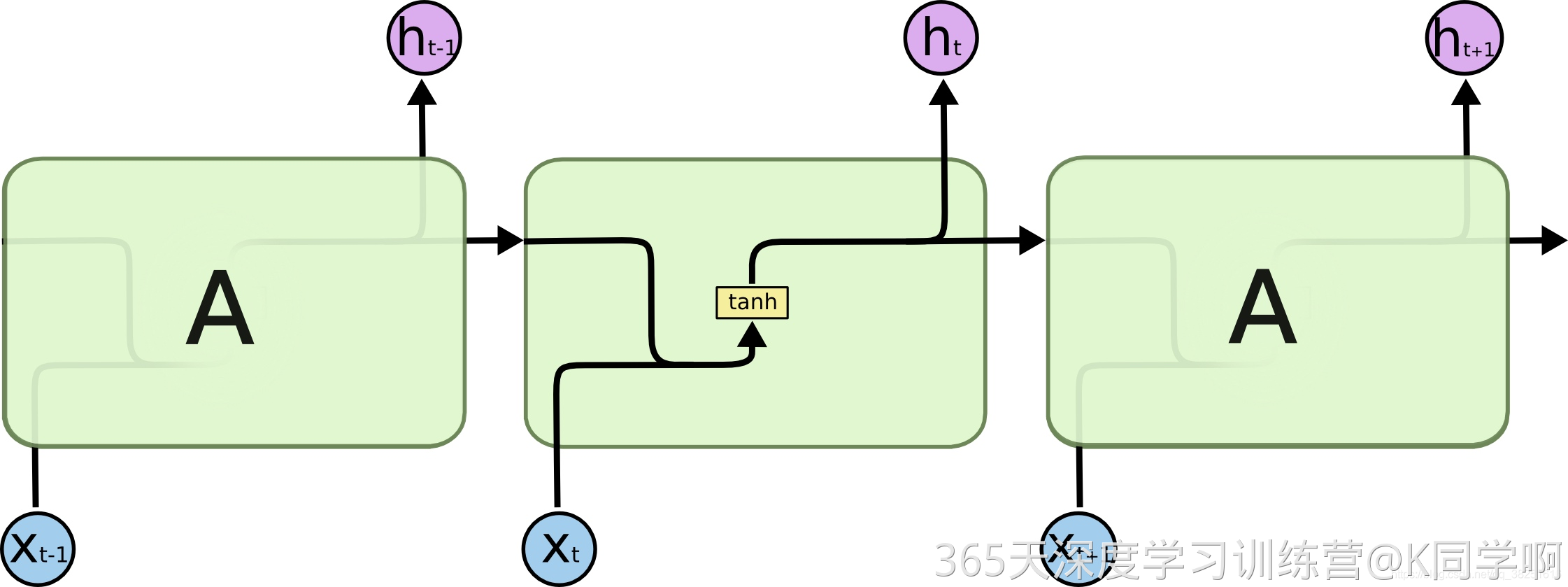
所有的循环神经网络都有着重复的神经网络模块形成链的形式。在普通的RNN中，重复模块结构非常简单，其结构如下：

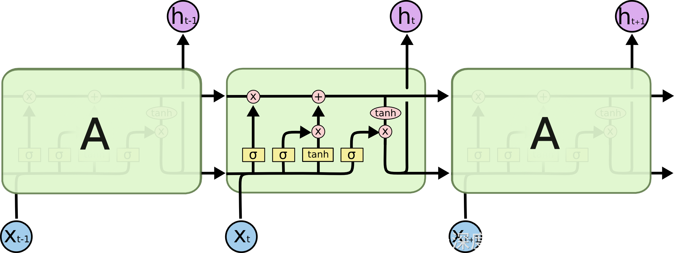
LSTM避免了长期依赖的问题。可以记住长期信息！LSTM内部有较为复杂的结构。能通过门控状态来选择调整传输的信息，记住需要长时间记忆的信息，忘记不重要的信息，其结构如下：

二：前期准备工作

1:导入数据

python 复制代码

import tensorflow as tf
import pandas as pd
import numpy as np

gpus = tf.config.list_physical_devices('GPU')
if gpus:
  tf.config.experimental.set_memory_growth(gpus[0], True)
  tf.config.set_visible_devices(gpus[0], 'GPU')

print(gpus)

df_1 = pd.read_csv("/content/drive/MyDrive/woodpine2.csv")

2:数据可视化

python 复制代码

import matplotlib.pyplot as plt
import seaborn as sns

plt.rcParams['savefig.dpi'] = 500 #图片像素
plt.rcParams['figure.dpi'] = 500 #分辨率
fig, ax = plt.subplots(1,3,constrained_layout=True, figsize=(14,3))

sns.lineplot(data = df_1['Tem1'],ax = ax[0])
sns.lineplot(data = df_1['CO 1'],ax = ax[1])
sns.lineplot(data = df_1['Soot 1'],ax = ax[2])
plt.show()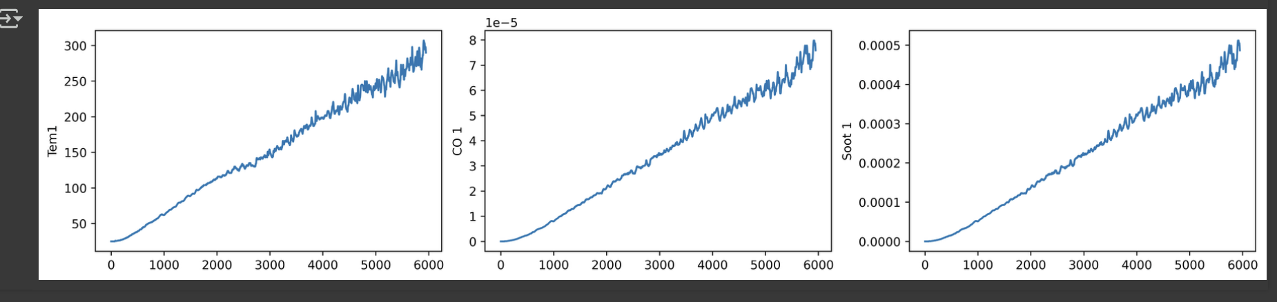

三：构建数据集

python 复制代码

dataFrame = df_1.iloc[:,1:]
dataFrame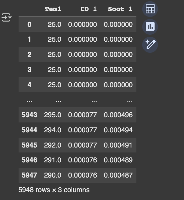

1:设置X,y

python 复制代码

width_X = 8
width_y= 1

取前8个时间段的Tem 1,CO 1,Soot 1为 X，第9个时间段的Tem1为y

python 复制代码

X = []
y = []

in_start = 0 

for _,_ in df_1.iterrows():
  in_end = in_start + width_X
  out_end = in_end + width_y
  if out_end < len(dataFrame):
    X_ = np.array(dataFrame.iloc[in_start:in_end,])
    X_ = X_.reshape((len(X_)*3))
    y_ = np.array(dataFrame.iloc[in_end:out_end,0])

    X.append(X_)
    y.append(y_)

  in_start += 1

X=np.array(X)
y = np.array(y)

X.shape,y.shape

2:归一化

python 复制代码

from sklearn.preprocessing import MinMaxScaler
scaler = MinMaxScaler(feature_range=(0, 1))
X_scaled = scaler.fit_transform(X)
X_scaled.shape

python 复制代码

X_scaled = X_scaled.reshape(len(X_scaled),width_X,3)
X_scaled.shape

3:划分数据集

python 复制代码

X_train = np.array(X_scaled[:5000]).astype('float64')
y_train = np.array(y[:5000]).astype('float64')
X_test = np.array(X_scaled[5000:]).astype('float64')
y_test = np.array(y[5000:]).astype('float64')

python 复制代码

X_train.shape

四：构建模型

python 复制代码

from tensorflow.keras.models import Sequential
from tensorflow.keras.layers import Dense, LSTM, Dropout, Bidirectional
from tensorflow.keras import Input

model_lstm = Sequential()
model_lstm.add(LSTM(64, activation='relu', input_shape=(X_train.shape[1],3), return_sequences=True))
model_lstm.add(LSTM(64, activation='relu'))
model_lstm.add(Dense(width_y))

五：模型训练

1:编译

python 复制代码

model_lstm.compile(optimizer=tf.keras.optimizers.Adam(1e-3), loss='mse')

2:训练

python 复制代码

history_lstm = model_lstm.fit(X_train, y_train, epochs=40, batch_size=64, validation_data=(X_test, y_test), validation_freq=1)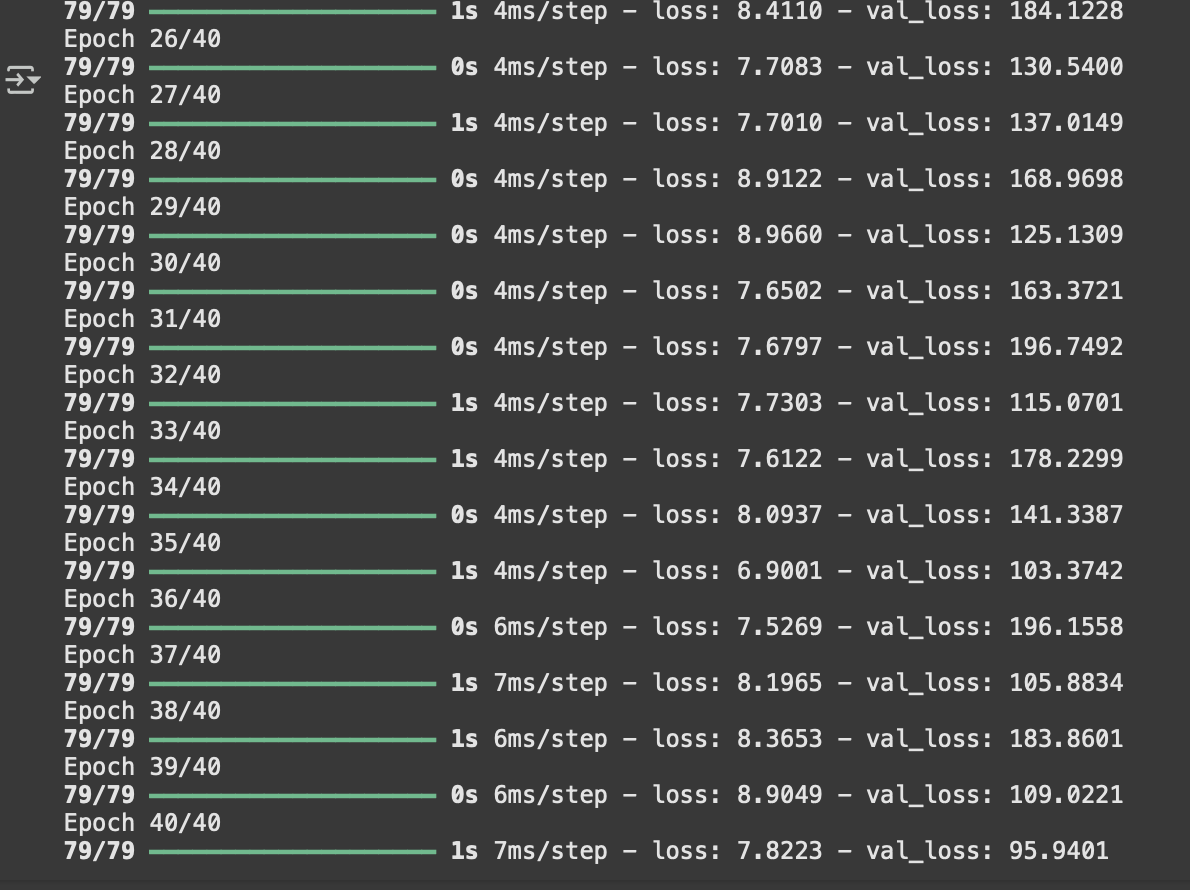

五：评估

1:loss图

python 复制代码

plt.rcParams['font.sans-serif'] = ['SimHei']
plt.rcParams['axes.unicode_minus'] = False
plt.figure(figsize = (5,3),dpi =120)

plt.plot(history_lstm.history['loss'],label = 'LSTM Training Loss')
plt.plot(history_lstm.history['val_loss'],label = 'LSTM Validation Loss')

plt.title('Training and Validation Loss')
plt.legend()
plt.show()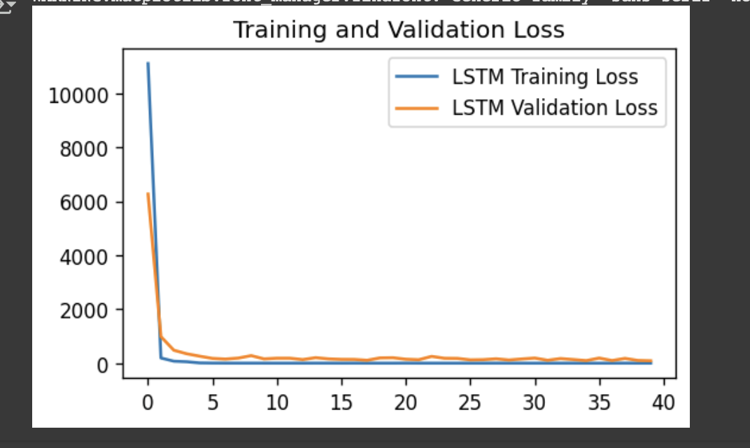

2:调用模型进行预测

python 复制代码

predicted_y_lstm = model_lstm.predict(X_test)
y_test_one = [i[0] for i in y_test]
predicted_y_lstm_one = [i[0] for i in predicted_y_lstm]

plt.figure(figsize = (5,3),dpi = 120)
plt.plot(y_test_one[:1000],color = 'red',label='true value')
plt.plot(predicted_y_lstm_one[:1000],color = 'blue',label='predicted value')
plt.title('Title')
plt.xlabel('X label')
plt.ylabel('Y label')
plt.legend()
plt.show()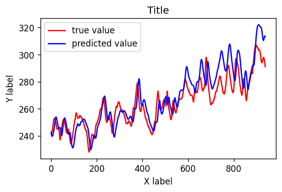

python 复制代码

from sklearn import metrics
RMSE_lstm = metrics.mean_squared_error(predicted_y_lstm,y_test)**0.5
R2_lstm = metrics.r2_score(predicted_y_lstm,y_test)
RMSE_lstm,R2_lstm