【R语言绘图】圈图绘制代码

绘制代码

rm(list = ls())

# 加载必要包
library(data.table)
library(circlize)
library(ComplexHeatmap)
library(rtracklayer)
library(GenomicRanges)
library(BSgenome)
library(GenomicFeatures)
library(dplyr)

### 数据准备阶段 ###
# 1. 读取染色体长度信息
df <- read.table('all_noContig.sizes', col.names = c('chr_id','chr_len'))

# 2. 读取基因组序列
genome <- readDNAStringSet("TG1.LG.fasta")

# 3. 计算GC含量（窗口：10kb，步长5kb）
window_size <- 10000
step <- 5000

gc_content <- lapply(names(genome), function(chr) {
  seq <- genome[[chr]]
  starts <- seq(1, length(seq) - window_size, by = step)
  ends <- starts + window_size
  gc <- sapply(1:length(starts), function(i) {
    subseq <- subseq(seq, starts[i], ends[i])
    sum(alphabetFrequency(subseq)[c("C","G")]) / window_size
  })
  data.frame(chrom = chr, start = starts, end = ends, gc = gc)
}) %>% bind_rows() %>%
  filter(!grepl("Contig", chrom)) %>%
  setNames(c('chr_id','bin_start','bin_end','gc'))

# 4. 读取基因密度数据
gc <- read.table('gene_counts.txt', 
                 col.names = c('chr_id','bin_start','bin_end','gene_count')) %>%
  filter(!grepl("Contig", chr_id))

# 5. 处理CDS注释数据
txdb <- makeTxDbFromGFF("TG1.gene.new.gff")
cds_ranges <- cds(txdb) %>% 
  as.data.frame() %>%
  dplyr::select(seqnames, start, end) %>%
  setNames(c('chr_id','bin_start','bin_end'))
pdf('circle.pdf')
### 绘图参数初始化 ###
circos.clear()
col_text <- 'grey20'

# 关键参数设置：统一轨道高度与边距
circos.par(
  gap.degree = 5,          # 染色体间空隙
  start.degree = 86,       # 起始角度
  track.height = 0.15,     # 统一轨道高度比例
  track.margin = c(0.01, 0.01), # 垂直边距压缩
  cell.padding = c(0,0,0,0),
  clock.wise = TRUE
)

# 初始化染色体布局
circos.initialize(
  factors = df$chr_id,
  xlim = cbind(rep(0, nrow(df)), df$chr_len)
)

### 绘图轨道绘制 ###
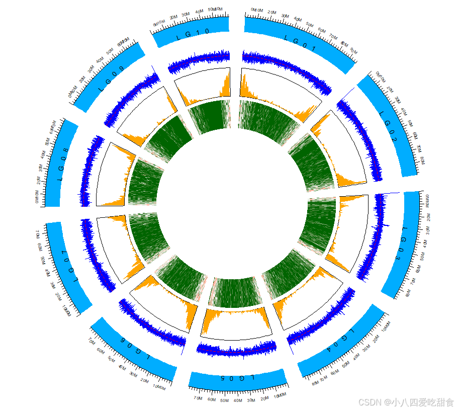
# 轨道1：染色体名称
circos.track(ylim = c(0, 1), panel.fun = function(x, y) {
  chr = CELL_META$sector.index
  circos.text(CELL_META$xcenter, CELL_META$ycenter, chr, 
              facing = "bending.inside", cex = 0.8)
}, bg.col = "#00ADFF", track.height = 0.08, bg.border = NA)

# 轨道2：刻度标签
brk <- seq(0, 100e6, by = 10e6)
circos.track(track.index = get.current.track.index(), 
             panel.fun = function(x, y) {
               circos.axis(h = "top", major.at = brk, 
                           labels = paste0(brk/1e6, "M"),
                           labels.cex = 0.5)
             }, bg.border = NA)
# 轨道4：GC含量
circos.genomicTrack(gc_content, panel.fun = function(region, value, ...) {
  circos.genomicLines(region, value, col = "blue", lwd = 0.5)
  circos.lines(CELL_META$cell.xlim, rep(mean(value[[1]]), 2), 
               col = "red", lty = 2)
}, track.height = 0.15, bg.border = NA)

# 轨道5：CDS密度
circos.genomicDensity(cds_ranges, col = c("orange"), 
                      bg.border = NA,
                      track.height = 0.15, window.size = 1e6)
# 轨道3：基因密度
color_genes <- colorRamp2(c(0, 6, 13), c("darkgreen", "white", "red"))
circos.genomicTrack(gc, panel.fun = function(region, value, ...) {
  circos.genomicRect(region, value, col = color_genes(value[[1]]), 
                     border = NA)
}, track.height = 0.15, bg.border = NA)

dev.off()
# 


### 图例添加 ###
lgd_list <- list(
  Legend(col_fun = color_genes, title = "Gene Density"),
  Legend(labels = c("GC Content", "Genome Average"), 
         type = "lines", 
         legend_gp = gpar(col = c("blue", "red"), lty = c(1,2))),
  Legend(col = "orange", title = "CDS Density", type = "points")
)

draw(lgd_list, x = unit(0.85, "npc"), just = "left")

### 图像输出 ###
circos.clear()

结果