Gmsh划分网格|四点矩形

先看下面这段官方自带脚本

/*********************************************************************
 *
 *  Gmsh tutorial 1
 *
 *  Variables, elementary entities (points, curves, surfaces), physical
 *  entities (points, curves, surfaces)
 *
 *********************************************************************/

// The simplest construction in Gmsh's scripting language is the
// `affectation'. The following command defines a new variable `lc':

lc = 1e-2;

// This variable can then be used in the definition of Gmsh's simplest
// `elementary entity', a `Point'. A Point is defined by a list of four numbers:
// three coordinates (X, Y and Z), and a characteristic length (lc) that sets
// the target element size at the point:

Point(1) = {0, 0, 0, lc};

// The distribution of the mesh element sizes is then obtained by interpolation
// of these characteristic lengths throughout the geometry. Another method to
// specify characteristic lengths is to use general mesh size Fields (see
// `t10.geo'). A particular case is the use of a background mesh (see `t7.geo').

// We can then define some additional points as well as our first curve.  Curves
// are Gmsh's second type of elementery entities, and, amongst curves, straight
// lines are the simplest. A straight line is defined by a list of point
// numbers. In the commands below, for example, the line 1 starts at point 1 and
// ends at point 2:

Point(2) = {.1, 0,  0, lc} ;
Point(3) = {.1, .3, 0, lc} ;
Point(4) = {0,  .3, 0, lc} ;

Line(1) = {1,2} ;
Line(2) = {3,2} ;
Line(3) = {3,4} ;
Line(4) = {4,1} ;

// The third elementary entity is the surface. In order to define a simple
// rectangular surface from the four curves defined above, a curve loop has first
// to be defined. A curve loop is a list of connected curves, a sign being
// associated with each curve (depending on the orientation of the curve):

Curve Loop(1) = {4,1,-2,3} ;

// We can then define the surface as a list of curve loops (only one here, since
// there are no holes--see `t4.geo'):

Plane Surface(1) = {1} ;

// At this level, Gmsh knows everything to display the rectangular surface 6 and
// to mesh it. An optional step is needed if we want to group elementary
// geometrical entities into more meaningful groups, e.g. to define some
// mathematical ("domain", "boundary"), functional ("left wing", "fuselage") or
// material ("steel", "carbon") properties.
//
// Such groups are called "Physical Groups" in Gmsh. By default, if physical
// groups are defined, Gmsh will export in output files only those elements that
// belong to at least one physical group. (To force Gmsh to save all elements,
// whether they belong to physical groups or not, set "Mesh.SaveAll=1;", or
// specify "-save_all" on the command line.)
//
// Here we define a physical curve that groups the left, bottom and right lines
// in a single group (with prescribed tag 5); and a physical surface with name
// "My surface" (with an automatic tag) containg the geometrical surface 1:

Physical Curve(5) = {1, 2, 4} ;
Physical Surface("My surface") = {1} ;

// Note that starting with Gmsh 3.0, models can be built using different
// geometry kernels than the default "built-in" kernel. By specifying
//
//   SetFactory("OpenCASCADE");
//
// any subsequent command in the .geo file would be handled by the OpenCASCADE
// geometry kernel instead of the built-in kernel. A rectangular surface could
// then simply be created with
//
//   Rectangle(2) = {.2, 0, 0, 0.1, 0.3};
//
// See tutorial/t16.geo for a complete example, and demos/boolean for more.
//+
Field[1] = Box;
//+
Delete Field [1];

以下是该Gmsh脚本代码的逐段解释：

---

1. 定义特征长度

lc = 1e-2;

• 作用 ：设置网格的特征长度为0.01，该值将影响后续生成的网格密度。
  取0.01时，如下：

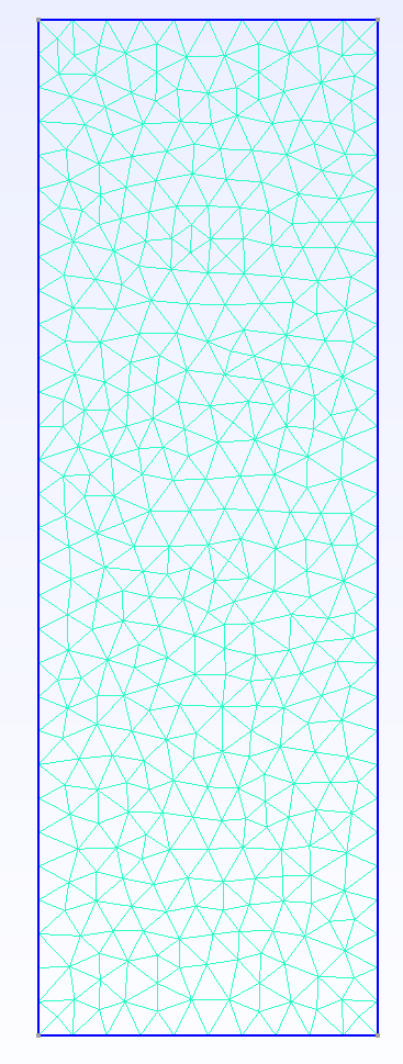
取0.1时，如下：

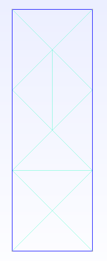
• 说明 ：lc 是局部网格尺寸的基准值，越小生成的网格越密。

---

2. 创建点（Points）

Point(1) = {0, 0, 0, lc};
Point(2) = {.1, 0,  0, lc};
Point(3) = {.1, .3, 0, lc};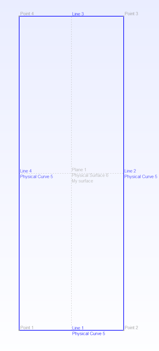
Point(4) = {0,  .3, 0, lc};

• 作用：在二维平面上定义四个点。
• 参数 ：Point(标签) = {X坐标, Y坐标, Z坐标, 特征长度}。
• 结果：四个点构成矩形的四个顶点（左下、右下、右上、左上）。

---

3. 创建线段（Lines）

Line(1) = {1, 2};  // 从点1到点2的线段
Line(2) = {3, 2};  // 从点3到点2的线段
Line(3) = {3, 4};  // 从点3到点4的线段
Line(4) = {4, 1};  // 从点4到点1的线段

• 作用：通过连接点生成四条线段。
• 注意 ：线段方向影响后续曲线环的定义，负号表示反向（例如 -2 表示线段2的反方向）。

---

4. 定义曲线环（Curve Loop）

Curve Loop(1) = {4, 1, -2, 3};

• 作用：将线段组合成闭合的环形，用于生成平面。
• 顺序 ：按闭合路径依次连接线段：
  1. 线段4（点4→点1）
  2. 线段1（点1→点2）
  3. 线段-2（点2→点3，反向线段2）
  4. 线段3（点3→点4）

---

5. 创建平面表面（Surface）

Plane Surface(1) = {1};

• 作用：通过曲线环1生成平面表面。
• 说明：此处定义了一个矩形区域，后续将在此区域内生成网格。

---

6. 定义物理实体（Physical Entities）

Physical Curve(5) = {1, 2, 4};
Physical Surface("My surface") = {1};

• 作用 ：将几何实体分组，用于后续仿真或导出。
  • 物理曲线5：包含线段1、2、4，代表模型的边界（例如左、下、右边）。
  • 物理表面"My surface"：包含表面1，代表整个矩形区域。
• 意义：物理实体用于在导出网格时标记不同区域（如边界条件、材料属性）。

---

7. 其他代码片段

Field[1] = Box;
Delete Field [1];

• 作用 ：尝试定义一个 Box 类型的场（用于控制网格尺寸），但随后被删除。
• 说明：这段代码可能是测试或误操作，实际未生效。

---

关键概念总结

1. 特征长度 lc：控制网格密度，值越小网格越密。
2. 曲线环方向：线段的正负号决定方向，确保闭合路径正确。
3. 物理实体 ：
   • 定义仿真中需要关注的区域（如边界、体积）。
   • 默认仅导出属于物理实体的网格单元。

---

生成的几何结构

• 一个矩形区域，左下角在原点 (0,0)，右上角在 (0.1, 0.3)。
• 物理曲线标记了左、下、右边界，物理表面标记了整个矩形区域。

通过此脚本，Gmsh将生成一个带有结构化网格的矩形，并仅导出标记的物理实体部分。