实验设计与分析（第6版，Montgomery)第3章单因子实验：方差分析3.11思考题3.4 R语言解题

本文是实验设计与分析（第6版，Montgomery著，傅珏生译) 第3章单因子实验：方差分析3.11思考题3.4 R语言解题。主要涉及单因子方差分析，正态性假设检验，残差与拟合值的关系图，LSD法。

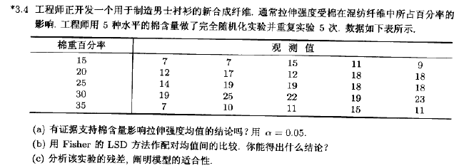
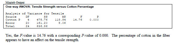
(a) Is there evidence to support the claim that cotton content affects the mean tensile strength? Use α = 0.05.

X<-c(7,7,15,11,9,12,17,12,18,18,14,19,19,18,18,19,25,22,19,23,7,10,11,15,11)

A<-factor(rep(1:5, each=5))

miscellany<-data.frame(X,A)

aov.mis<-aov(X~A, data=miscellany)

> summary(aov.mis) Df Sum Sq Mean Sq F value Pr(>F)

A 4 475.8 118.94 14.76 9.13e-06 ***

Residuals 20 161.2 8.06

---

Signif. codes:

0 '***' 0.001 '**' 0.01 '*' 0.05 '.' 0.1 ' ' 1

Yes, the F -value is 14.76 with a corresponding P-value of 0.000. The percentage of cotton in the fiber appears to have an affect on the tensile strength.

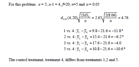
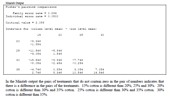
(b) Use the Fisher LSD method to make comparisons between the pairs of means. What conclusions can you draw?

install.packages("DescTools")

library(DescTools)

PostHocTest(aov.mis,method = "lsd")

> PostHocTest(aov.mis,method = "lsd")

Posthoc multiple comparisons of means : Fisher LSD

95% family-wise confidence level

$A

diff lwr.ci upr.ci pval

2-1 5.6 1.8545482 9.3454518 0.00541 **

3-1 7.8 4.0545482 11.5454518 0.00031 ***

4-1 11.8 8.0545482 15.5454518 2.1e-06 ***

5-1 1.0 -2.7454518 4.7454518 0.58375

3-2 2.2 -1.5454518 5.9454518 0.23471

4-2 6.2 2.4545482 9.9454518 0.00251 **

5-2 -4.6 -8.3454518 -0.8545482 0.01859 *

4-3 4.0 0.2545482 7.7454518 0.03754 *

5-3 -6.8 -10.5454518 -3.0545482 0.00116 **

5-4 -10.8 -14.5454518 -7.0545482 7.0e-06 ***

---

Signif. codes: 0 '***' 0.001 '**' 0.01 '*' 0.05 '.' 0.1 ' ' 1

#P.92 3.4題

y1 <- c(7,7,15,11,9)

y2 <- c(12,17,12,18,18)

y3 <- c(14,18,18,19,19)

y4 <- c(19,25,22,19,23)

y5 <- c(7,10,11,15,11)

y <- c(y1,y2,y3,y4,y5)

group <- c(rep(1,5),rep(2,5),rep(3,5),rep(4,5),rep(5,5))

a <- 5

n <- length(y1)

N <- length(y)

tapply(y,group,sum)

> tapply(y,group,sum)

1 2 3 4 5

49 77 88 108 54

tapply(y,group,mean)

> tapply(y,group,mean) 1 2 3 4 5

9.8 15.4 17.6 21.6 10.8

y.sum <- sum(y)

y.ave <- y.sum/N

> y.sum[1]

376

SST <- sum(y^2) - y.sum^2/N

> SST[1]

636.96

SS.treatments <- sum((tapply(y,group,sum))^2)/n - y.sum^2/N

> SS.treatments[1]

475.76

SSE <- SST - SS.treatments

> SSE

1\] 161.2 F0 \<- (SS.treatments/(a-1))/(SSE/(N-a)) \> F0 \[1\] 14.75682 qf(0.95,a-1,N-a) #critical value \> qf(0.95,a-1,N-a) #critical value \[1\] 2.866081 1. pf(F0,a-1,N-a) #P-value \> 1-pf(F0,a-1,N-a) #P-value \[1\] 9.127937e-06 data \<- data.frame(y=y, group=factor(group)) fit \<- lm(y\~group, data) anova(fit) \> anova(fit)Analysis of Variance Table Response: y Df Sum Sq Mean Sq F value Pr(\>F) group 4 475.76 118.94 14.757 9.128e-06 \*\*\* Residuals 20 161.20 8.06 --- Signif. 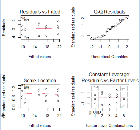codes: 0 '\*\*\*' 0.001 '\*\*' 0.01 '\*' 0.05 '.' 0.1 ' ' 1 #postscript("original.eps",height=5,width=5,horizontal=F) par(mfrow=c(2,2)) plot(fit) #residual plots #dev.off()