Ribbon过滤器整体看是一个矩阵构建与矩阵乘法,RocksDB中对它的实现是进行了合理的空间、时间上的优化的。
符号
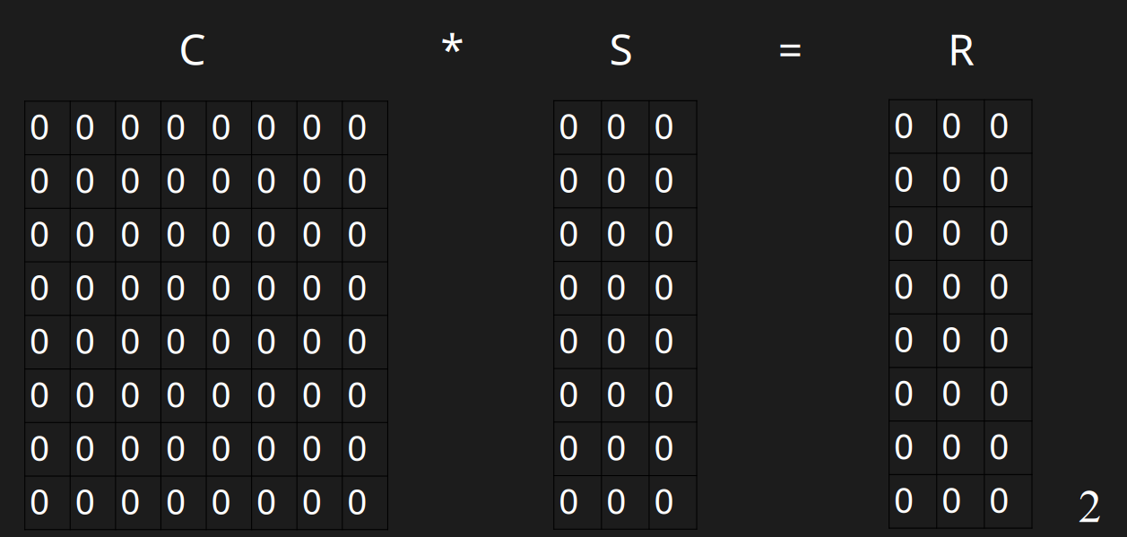
整个过滤器都和矩阵计算CS=R相关,C是\(n*n\)矩阵,S是\(n*m\)矩阵,R是\(n*m\)矩阵。
这里为了方便讨论定义:三个哈希函数s(x),c(x),r(x),s是start函数,c是coeff函数,r是result函数。其中c的返回值是一个定长二进制整数,比如c(x)返回0010,那么c(x)返回的整数是长度为w=4的二进制整数。
此外为了方便讨论,我们假定n=8, m=3,h(x)为s(x)个0拼接c(x)拼接n-w-s(x)个0。比如:
| key | s(x) | c(x) | r(x) | h(x) |
|---|---|---|---|---|
| u | 0 | 1000 | 000 | 1000 0000 |
| v | 0 | 1100 | 111 | 1100 0000 |
| w | 0 | 1010 | 100 | 1010 0000 |
| x | 3 | 1000 | 101 | 000 1000 0 |
| y | 0 | 1001 | 111 | 1001 0000 |
构建过程
构建过程本质上是解一个CS=R的矩阵乘法。C和R是由插入的键构建的,S是C和R解出来的。这里定义的矩阵乘法是:
\c_{ij} = \\bigoplus_{k=1}\^{n} (a_{ik} \\land b_{kj}) \\
与原本的矩阵乘法非常相似,就是乘法变成逻辑与,加法编程逻辑xor罢了。
\c_{ij} = \\sum_{k=1}\^{n} a_{ik} b_{kj} \\
初始化
初始化,默认所有值为0
插入过程
python
    def leading_zeros_count(self, vec: np.matrix):
        for i in range(vec.shape[1]):
            if vec[0, i] != 0:
                return i
        return vec.shape[1]

    def banding_add(self, h, resultrow):
        print(h, resultrow)
        while True:
            start = self.leading_zeros_count(h)
            if np.all(h[0] == 0):
                if np.all(resultrow[0] == 0):
                    break
                else:
                    raise ValueError("cannot insert this row")
            elif np.all(self.coeff[start] == 0): # 如果start这一行全是0,就把这一行赋值为coeffrow
                self.coeff[start] = h
                self.result[start] = resultrow
                break
            else:
                h = self.row_xor(h, self.coeff[start])
                resultrow = self.row_xor(resultrow, self.result[start])
        print(self.coeff)
        print(self.result)
插入u
插入u的时候,此时它开头的0的数量是0,需要插入到第0行。第0行都是0,直接插入即可。

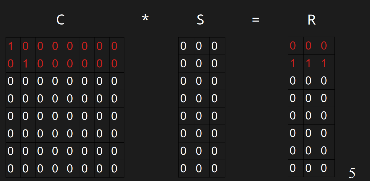
插入v
插入v的时候,此时它开头的0的数量是1,需要插入到第0行。第0行已经有值了,h(v)=11000000与r(v)=111分别与第0行异或,得到01000000与111。此时它开头的0的数量是1,需要插入到第1行,可以直接插入。
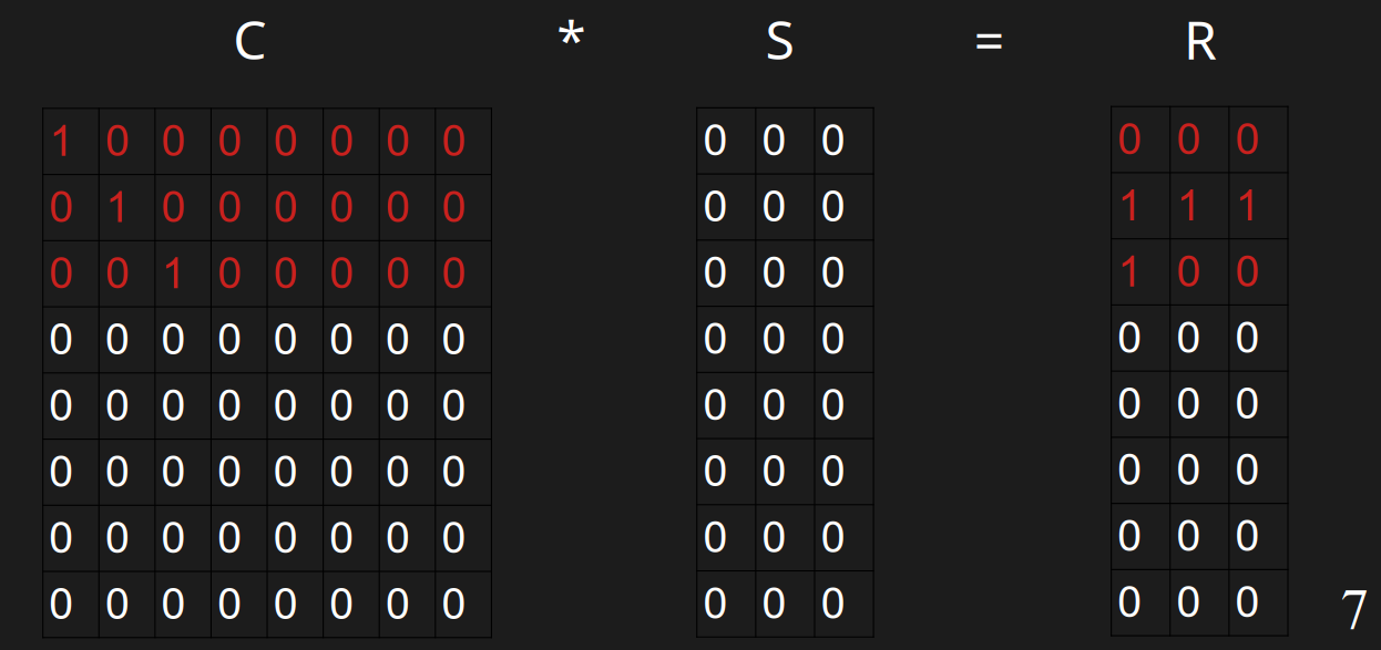
插入w
插入w的时候,h(w)=10100000,r(w)=100,此时它开头的0的数量是0,需要插入到第0行。发现第0行有值了,分别与第0行异或,得到00100000与100,此时它开头的0的数量是2,此时需要插入到第2行。
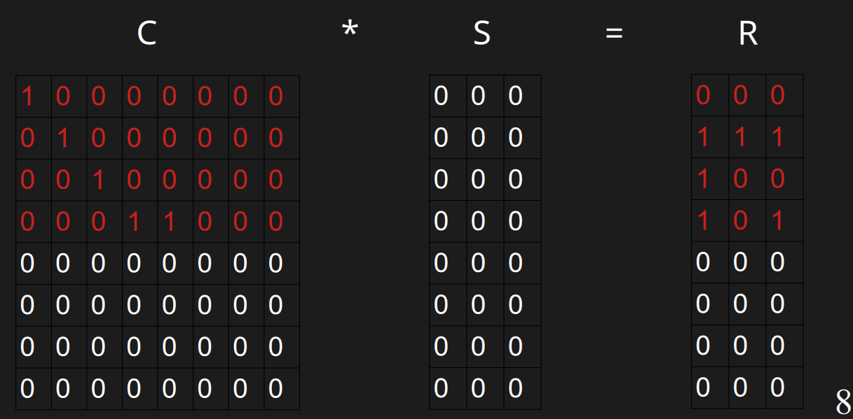
插入x
插入x的时候,h(x)=00011000,r(x)=100,此时它开头的0的数量是3,需要插入到第3行,插入到第3行。
插入y
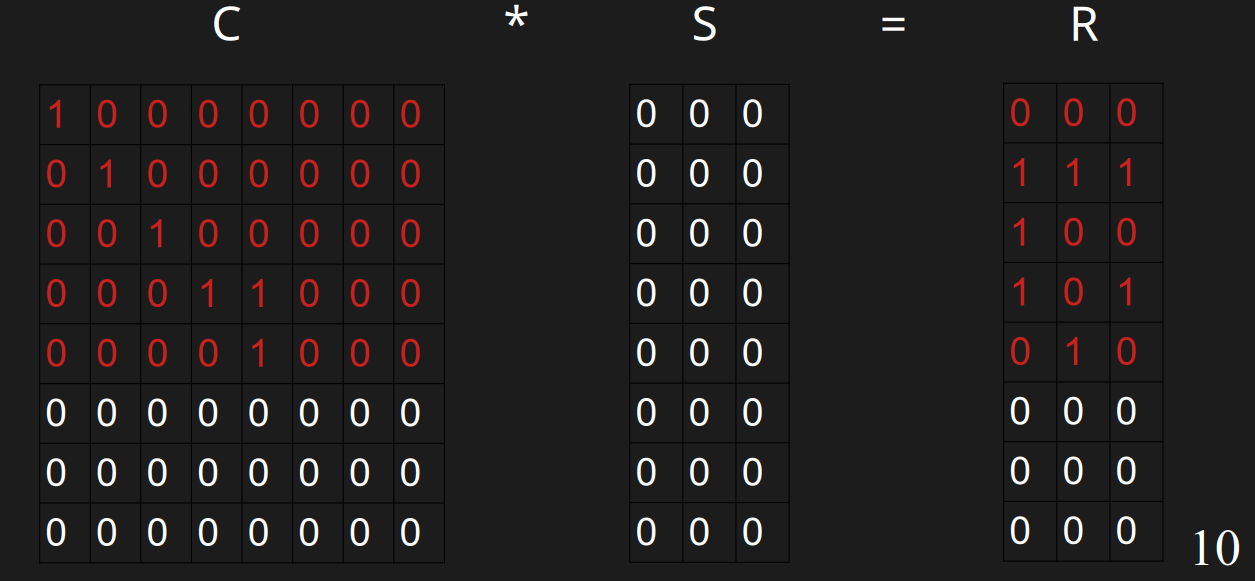
插入y的时候,h(w)=10010000,r(w)=111,此时它开头的0的数量是0,需要插入到第0行。
发现第0行有值了,分别与第0行异或,得到00010000与111,此时它开头的0的数量是3,此时需要插入到第3行。
发现第3行有值了,分别与第3行异或,得到00001000与010,此时它开头的0的数量是4,此时需要插入到第4行。
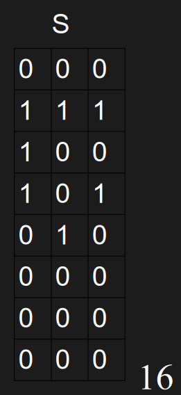
解矩阵S
现在有C和R了,可以用线性代数的方法解S的值。但是由于C是上三角矩阵,且中间长度w=4的01串以外的地方都是0,所以我们可以从下往上计算,且只需要看其中4个值。
解S的第4行
解这一行本质上是计算\(00001000*S=010\),即:
\0 \\and S_{0,0} \\oplus 0 \\and S_{1,0} \\oplus 0 \\and S_{2,0} \\oplus 0 \\and S_{3,0} \\oplus 1 \\and S_{4,0} \\oplus 0 \\and S_{5,0} \\oplus 0 \\and S_{6,0} \\oplus 0 \\and S_{7,0} = 0 \\
\0 \\and S_{0,1} \\oplus 0 \\and S_{1,1} \\oplus 0 \\and S_{2,1} \\oplus 0 \\and S_{3,1} \\oplus 1 \\and S_{4,1} \\oplus 0 \\and S_{5,1} \\oplus 0 \\and S_{6,1} \\oplus 0 \\and S_{7,1} = 1 \\
\0 \\and S_{0,2} \\oplus 0 \\and S_{1,2} \\oplus 0 \\and S_{2,2} \\oplus 0 \\and S_{3,2} \\oplus 1 \\and S_{4,2} \\oplus 0 \\and S_{5,2} \\oplus 0 \\and S_{6,2} \\oplus 0 \\and S_{7,2} = 0 \\
由于C是上三角矩阵,且其中只有连续的4个wit可能为1,其他都为0,所以上面的计算可以化简为:
\1 \\and S_{4,0} \\oplus 0 \\and S_{5,0} \\oplus 0 \\and S_{6,0} \\oplus 0 \\and S_{7,0} = 0 \\
\1 \\and S_{4,1} \\oplus 0 \\and S_{5,1} \\oplus 0 \\and S_{6,1} \\oplus 0 \\and S_{7,1} = 1 \\
\1 \\and S_{4,2} \\oplus 0 \\and S_{5,2} \\oplus 0 \\and S_{6,2} \\oplus 0 \\and S_{7,2} = 0 \\
由于C的最后三行是0,所以进一步化简为:
\1 \\and S_{4,0} = 0 \\
\1 \\and S_{4,1} = 1 \\
\1 \\and S_{4,2} = 0 \\
很容易解出来S的第四行

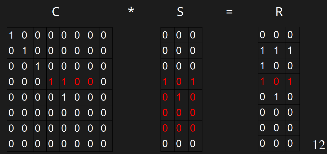
解S的第3行
计算
\0 \\and S_{0,0} \\oplus 0 \\and S_{1,0} \\oplus 0 \\and S_{2,0} \\oplus 1 \\and S_{3,0} \\oplus 1 \\and S_{4,0} \\oplus 0 \\and S_{5,0} \\oplus 0 \\and S_{6,0} \\oplus 0 \\and S_{7,0} = 1 \\
\0 \\and S_{0,1} \\oplus 0 \\and S_{1,1} \\oplus 0 \\and S_{2,1} \\oplus 1 \\and S_{3,1} \\oplus 1 \\and S_{4,1} \\oplus 0 \\and S_{5,1} \\oplus 0 \\and S_{6,1} \\oplus 0 \\and S_{7,1} = 0 \\
\0 \\and S_{0,2} \\oplus 0 \\and S_{1,2} \\oplus 0 \\and S_{2,2} \\oplus 1 \\and S_{3,2} \\oplus 1 \\and S_{4,2} \\oplus 0 \\and S_{5,2} \\oplus 0 \\and S_{6,2} \\oplus 0 \\and S_{7,2} = 1 \\
由于C是上三角矩阵,且其中只有连续的4个bit可能为1,其他都为0,所以上面的计算可以化简为:
\1 \\and S_{3,0} \\oplus 1 \\and S_{4,0} \\oplus 0 \\and S_{5,0} \\oplus 0 \\and S_{6,0} = 1 \\
\1 \\and S_{3,1} \\oplus 1 \\and S_{4,1} \\oplus 0 \\and S_{5,1} \\oplus 0 \\and S_{6,1} = 0 \\
\1 \\and S_{3,2} \\oplus 1 \\and S_{4,2} \\oplus 0 \\and S_{5,2} \\oplus 0 \\and S_{6,2} = 1 \\
容易算出S的第3行是101
以此类推,计算完S
查询过程
查询过程即判断表达式\(h(x)S=r(x)\)。
查询\(h(a)=11000000\)与\(r(a)=110\),\(h(a)S=111\),与r(a)不同,判定为不存在,查询结果正确
查询\(h(y)=10010000\)与\(r(y)=111\),\(h(y)S=101\),与r(y)不同,出现假阴性
查询\(h(b)=01000000\)与\(r(b)=111\),得到101,与r(b)不同,出现假阳性
查询\(h(u)=11000000\)与\(r(u)=111\),得到111,与r(u)相同,判定为存在,结果正确
优化
矩阵存储优化
可以发现,ribbon过滤器完全可以用一个\(w*n\)的矩阵表示整个C,并且构建完S后完全可以丢弃C和R,所以只会在构建过中存在临时的空间消耗。
构建、查询耗时优化
可以发现h(x)只有中间连续w个bit是有用的,所以查询时可以遍历S中的w行即可。
假阳性率定制
假阳性率是\(2^{-w}\),至于如何定制,这是论文中的内容了,如图,我们将w个 bit 连续存放,每m个w bit 为一组。所以整体看是 column-major 的,而每一组实际上是 row-major 的。这种混合方式称为 ICML(Interleaved Column-MajorLayout)
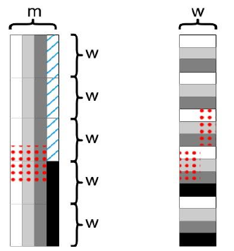
代码中,我们还需要特殊处理跨组(图中红点部分)的问题。对于 ICML 开始一段不足m列的特殊情况(图中蓝色斜线部分),我们可以忽略它。这样我们就可以存储 7、9、10bit 一行的矩阵。平均 3.4bit 一行的矩阵也是可行的,图中m = 4,但是前面三段都是使用m = 3,这样平均就是 3.4bit 一行了。
提防假阴性
从前面查询的例子我们可以发现,过滤器存在假阴性,即实际插入位置不在\[s(x),s(x)+w-1\]范围内,这是要避免的。为了确保假阴性率极低,需要多分配一些内存。比如插入t个key,那么实际要分配的行数是需要多于t的。具体的假阴性率真不知道怎么算,在代码中是设置为一个值来规避的。这个值是
\ 1-0.0251 + ln(t) \* 1.4427 \* 0.0083或1-0.0176 + ln(t) \* 1.4427 \* 0.0038; \\
算法导论有关于线性探测哈希表的讨论。如果w=64,那么期望探测到64次,load-factor需要是\(64=1/(1-a)\),解出来loadfactor为63/64,即0.98,而这个公式在\(t=30,000,000\)时算出来是0.83左右