目录
1963年,Lorenz发现了第一个混沌吸引子------Lorenz系统,从此揭开了混沌研究的序幕。
Lorenz 3 模型定义
Lorenz 1963 模型是描述大气对流的一个简化系统,具有混沌特性,是非线性动力系统研究的经典模型之一。
该系统由三个常微分方程组成:
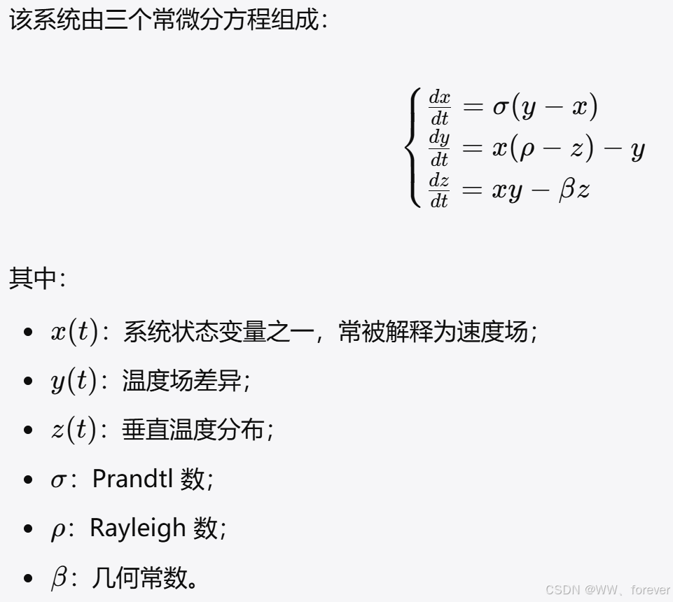
其中:
- ( x(t) ):系统状态变量之一,常被解释为速度场;
- ( y(t) ):温度场差异;
- ( z(t) ):垂直温度分布;
- ( \sigma ):Prandtl 数;
- ( \rho ):Rayleigh 数;
- ( \beta ):几何常数。
Lorenz模型已经成为混沌领域的经典模型,系统中三个参数的选择对系统会不会进入混沌状态起着重要的作用。
常用参数(具有混沌性)
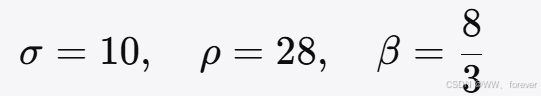
Lorenz 系统的行为高度依赖参数,例如:
| 参数组合 | 吸引子形态 | 案例图形 |
|---|---|---|
| ρ < 1 | Lorenz 系统在 𝜌<1 时,原点是唯一稳定点,所有轨道都会收敛到原点,系统不出现振荡或混沌。 | 轨道从初始点缓慢收敛到原点,轨迹几乎不动。(ρ=0.5<1)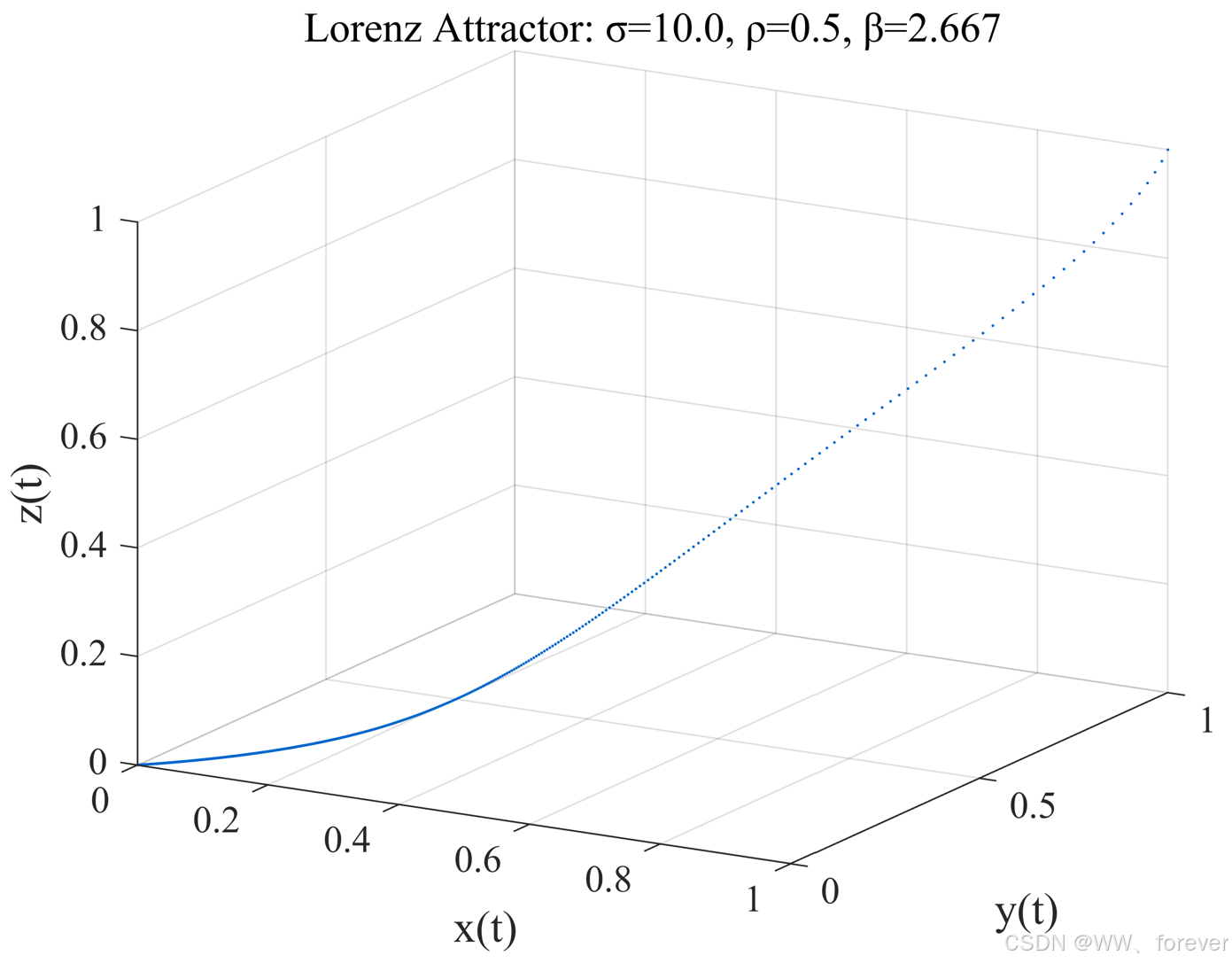 |
| ρ ≈ 10 | 出现两个稳定平衡点(非混沌),轨道会围绕其中一个平衡点收敛,表现为规则螺旋 | 轨道围绕两个点之间螺旋收敛,看不到明显的"蝴蝶形"混沌结构。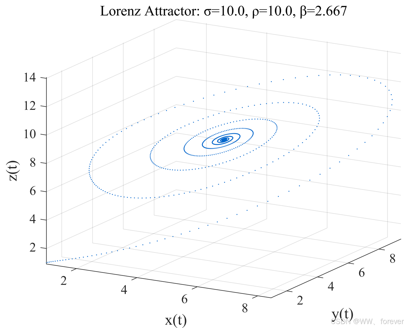 |
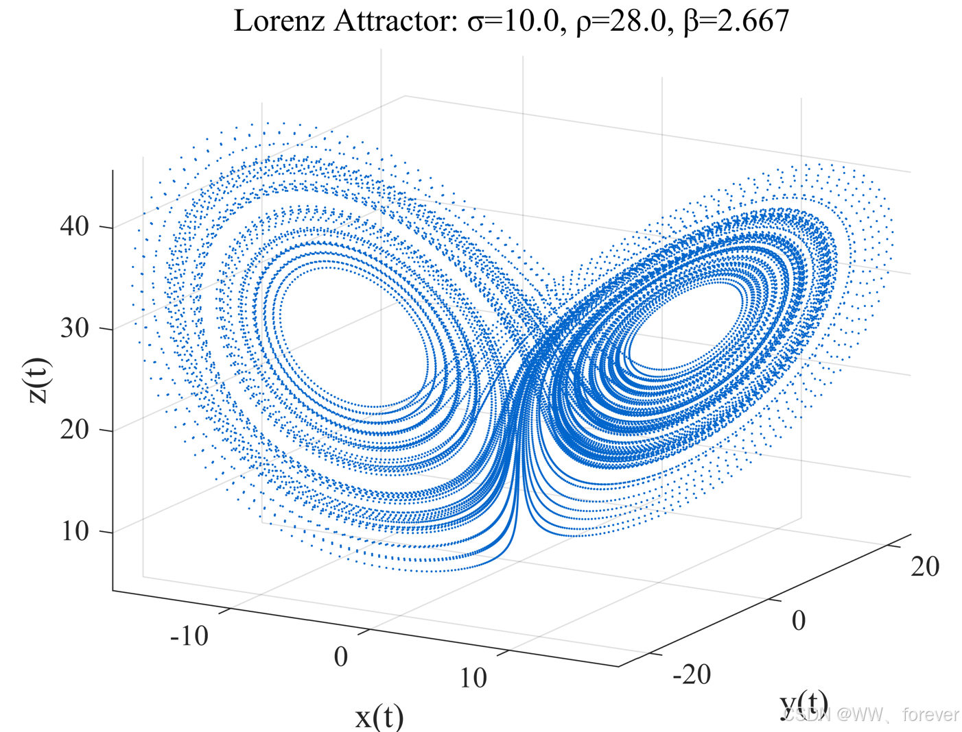
| ρ = 28 | 出现混沌吸引子(蝴蝶形) | Lorenz 系统最经典的混沌参量,轨道在两个"翅膀"之间不可预测地跳跃,形成典型混沌吸引子。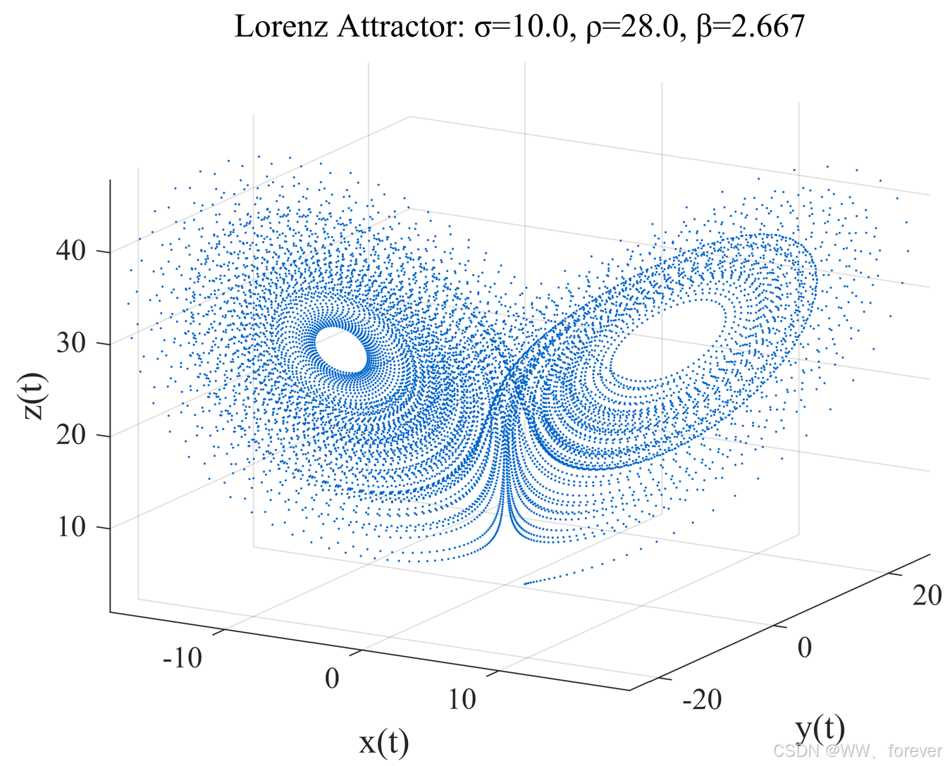 |
| ρ > 100 | 系统变得更混乱,吸引子形状更复杂 | 两个"翅膀"结构非常清晰,但比 𝜌=28 时范围更广、点分布更散,Z 方向振幅超过 200。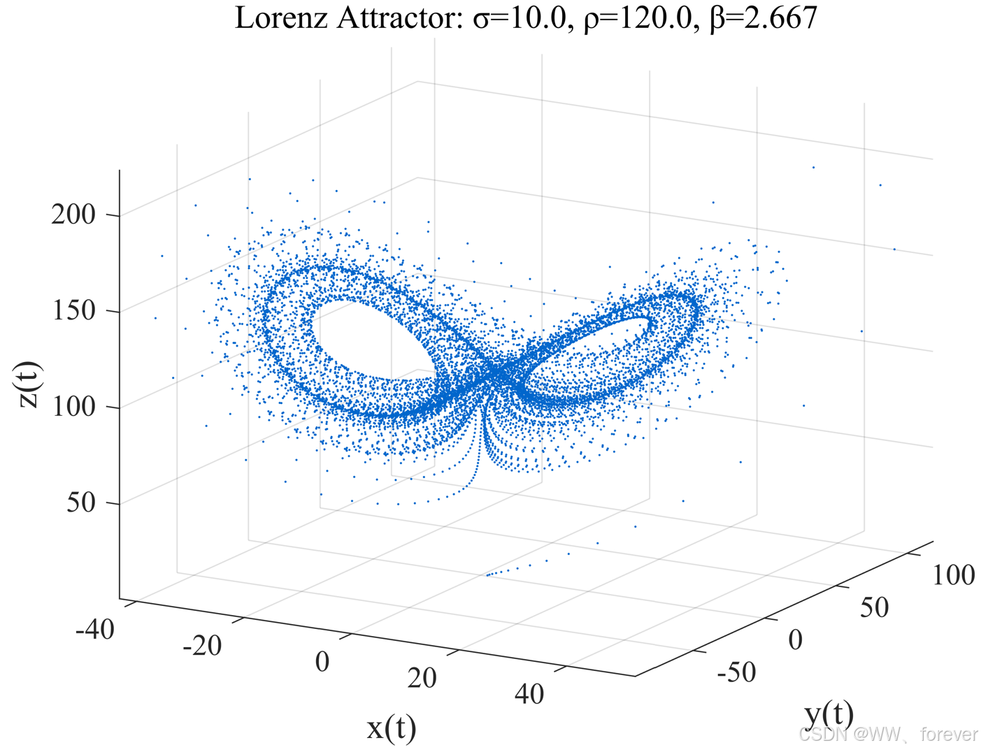 |
MATLAB代码
以下 MATLAB 代码将:
- 定义 Lorenz 系统;
- 使用
ode45数值积分; - 绘制 3D 演化轨迹
运行以下代码后,会得到一个立体的"蝴蝶型"轨迹图,显示 Lorenz 系统在混沌参数 下的演化行为。
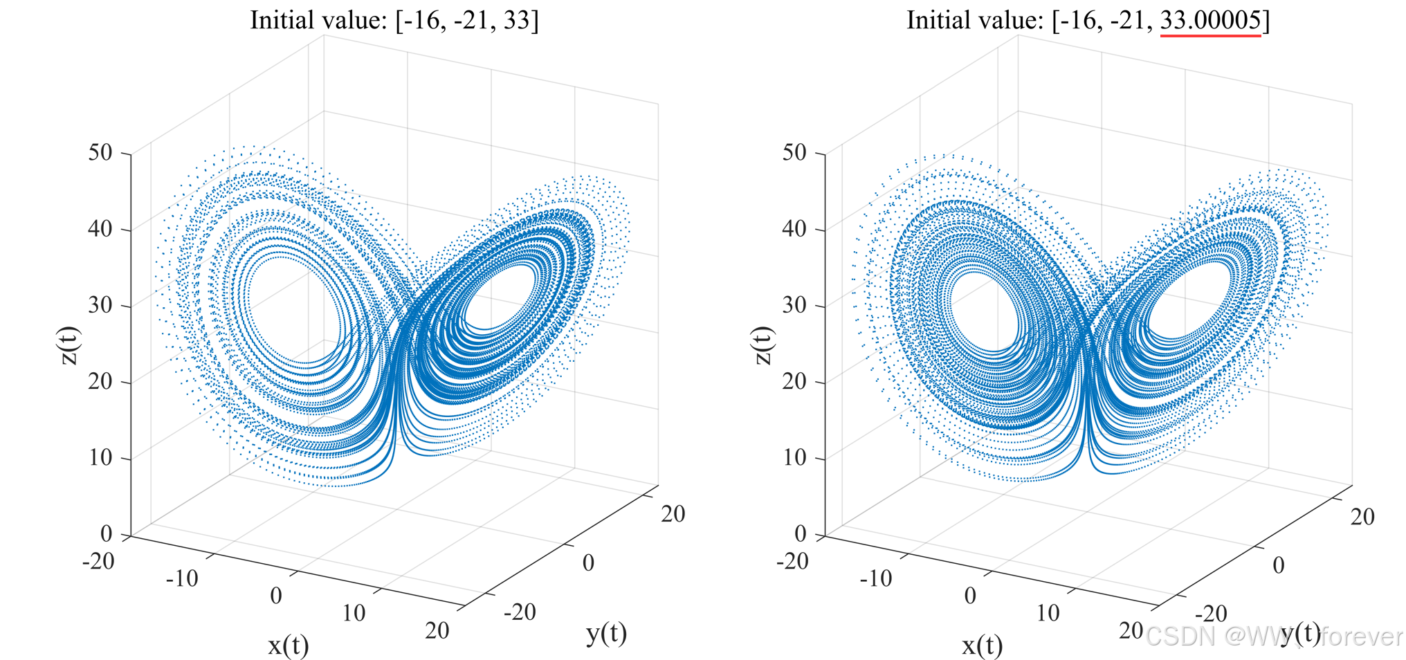
- 渐近吸引子 ------ 虽然初始点不同,但轨迹最终会在两个"翅膀"之间跳动;
- 对初始值敏感 ------ 稍微改变初值也会导致完全不同的轨迹;
完整matlab代码如下:
matlab
%% Lorenz 3D 系统演化轨迹绘制
clear;
clc;
close all;
pathFigure = "..\Figures\";
%% 参数设置
sigma = 10;
rho = 28;
beta = 8/3;
%% 时间设置
tspan = [0 100]; % 积分时间
dt = 0.005; % 步长
t = tspan(1):dt:tspan(2);
%% 初始条件
x0 = [-16, -21, 33]; % 可试试 [1, 1, 1] 或其他值
%% 积分
[t_out, x_out] = ode45(@(t,x) lorenz3(t,x,sigma,rho,beta), t, x0);
%% 提取变量
x = x_out(:,1);
y = x_out(:,2);
z = x_out(:,3);
%% 3D 轨迹图
figure('Name','Lorenz Attractor','Color','w');
plot3(x, y, z, '.', 'MarkerSize', 3, 'Color', [0 0.4 0.8]);
set(gca, 'FontSize', 12, 'FontName', 'Times New Roman');
xlabel('x(t)', 'FontSize', 14, 'FontName', 'Times New Roman');
ylabel('y(t)', 'FontSize', 14, 'FontName', 'Times New Roman');
zlabel('z(t)', 'FontSize', 14, 'FontName', 'Times New Roman');
grid on;
title(sprintf('Lorenz Attractor: σ=%.1f, ρ=%.1f, β=%.3f', sigma, rho, beta))
view(30, 20); % 设置视角
axis tight
str= strcat(pathFigure, "Fig.1", '.tiff');
print(gcf, '-dtiff', '-r600', str);
%%
figureUnits = 'centimeters';
figureWidth = 27;
figureHeight = 12;
figureHandle = figure;
set(gcf, 'Units', figureUnits, 'Position', [0 0 figureWidth figureHeight]);
subplot(1,2,1);
plot3(x, y, z, '.', 'MarkerSize', 2);
set(gca, 'FontSize', 12, 'FontName', 'Times New Roman');
xlabel('x(t)', 'FontSize', 14, 'FontName', 'Times New Roman');
ylabel('y(t)', 'FontSize', 14, 'FontName', 'Times New Roman');
zlabel('z(t)', 'FontSize', 14, 'FontName', 'Times New Roman');
grid on;
title('Initial value: [-16, -21, 33]');
view(30, 20); % 设置视角
set(gca,'Layer','top');
% 改变初值
x0_2 = [-16, -21, 33.00005];
[~, x2] = ode45(@(t,x) lorenz3(t,x,sigma,rho,beta), t, x0_2);
subplot(1,2,2);
plot3(x2(:,1), x2(:,2), x2(:,3), '.', 'MarkerSize', 2);
set(gca, 'FontSize', 12, 'FontName', 'Times New Roman');
xlabel('x(t)', 'FontSize', 14, 'FontName', 'Times New Roman');
ylabel('y(t)', 'FontSize', 14, 'FontName', 'Times New Roman');
zlabel('z(t)', 'FontSize', 14, 'FontName', 'Times New Roman');
grid on;
title('Initial value: [-16, -21, 33.00005]');
view(30, 20); % 设置视角
set(gca,'Layer','top');
str= strcat(pathFigure, "Fig.2", '.tiff');
print(gcf, '-dtiff', '-r600', str);
%% 函数定义
function dxdt = lorenz3(~, x, sigma, rho, beta)
dxdt = zeros(3,1);
dxdt(1) = sigma * (x(2) - x(1));
dxdt(2) = x(1) * (rho - x(3)) - x(2);
dxdt(3) = x(1) * x(2) - beta * x(3);
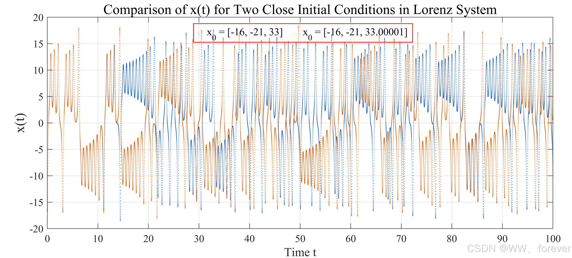
end对比两个初始值非常接近的 Lorenz 系统,分别绘制它们的 𝑥(𝑡) 时间序列,结果如下:
虽然初始值差异极小,但在一段时间后轨迹迅速分离,这正是 混沌系统敏感依赖初始条件(蝴蝶效应) 的体现
相应MATLAB实现代码如下:
matlab
x0_1 = [-16, -21, 33];
x0_2 = [-16, -21, 33.00001];  % 微小扰动

% 数值求解
[t1, x1] = ode45(@(t,x) lorenz3(t,x,sigma,rho,beta), t, x0_1);
[t2, x2] = ode45(@(t,x) lorenz3(t,x,sigma,rho,beta), t, x0_2);

% 提取 x 分量
x1_series = x1(:,1);
x2_series = x2(:,1);

% 绘图:对比 x(t) 时间序列
figure('Name','Lorenz x(t) Comparison','Color','w', 'Position', [100, 100, 1000, 400]);

plot(t1, x1_series, '.', 'MarkerSize', 2, 'Color', [0.1 0.4 0.8]); hold on;
plot(t2, x2_series, '.', 'MarkerSize', 2, 'Color', [0.9 0.4 0]);
set(gca, 'FontSize', 12, 'FontName', 'Times New Roman');
hl = legend('x_0 = [-16, -21, 33]', 'x_0 = [-16, -21, 33.00001]');
set(hl, 'NumColumns', 2, 'box', 'off', 'FontName', 'Times New Roman', 'FontSize', 12,'Location','north');
grid on;
xlim([0, max(t)]);

xlabel('Time t', 'FontSize', 14, 'FontName', 'Times New Roman');
ylabel('x(t)', 'FontSize', 16, 'FontName', 'Times New Roman');
title('Comparison of x(t) for Two Close Initial Conditions in Lorenz System', 'FontSize', 16, 'FontName', 'Times New Roman');
set(gca,'Layer','top');

str= strcat(pathFigure, "Fig.3", '.tiff');
print(gcf, '-dtiff', '-r600', str);