首先说明:arma 用于心电图不一定合适,只是手头正好有这个数据
python
import json
import numpy as np
import pandas as pd
import matplotlib.pyplot as plt
from statsmodels.tsa.stattools import adfuller, acf, pacf
from statsmodels.tsa.arima.model import ARIMA # ARMA是ARIMA的特殊情况(d=0)
from statsmodels.graphics.tsaplots import plot_acf, plot_pacf
from sklearn.metrics import mean_squared_error
# 设置中文字体
plt.rcParams["font.family"] = ["SimHei", "Microsoft YaHei"]
plt.rcParams['axes.unicode_minus'] = False # 解决负号显示问题
# 1. 加载并解析心电图数据
def load_ecg_data(file_path):
with open(file_path, 'r', encoding='utf-8') as f:
data = json.load(f) # 加载JSON数据
# 转换为DataFrame,每个通道作为一列
ecg_df = pd.DataFrame()
for channel in data:
ch_name = channel['channel']
# 检查数据长度
if len(channel['value']) != ecg_df.index.size and not ecg_df.empty:
print(f"警告:通道 {ch_name} 的数据长度与其他通道不一致,已跳过。")
continue
ecg_df[ch_name] = channel['value']
# 重置索引
ecg_df = ecg_df.reset_index(drop=True)
return ecg_df
# 加载数据(请替换为实际文件路径)
ecg_data = load_ecg_data('hisdata.txt')
print(f"数据形状:{ecg_data.shape},包含通道:{ecg_data.columns.tolist()}")
# 2. 数据预处理与可视化(以通道"I"为例)
ch = 'I' # 选择分析的通道
ecg_series = ecg_data[ch].copy() # 提取时序数据
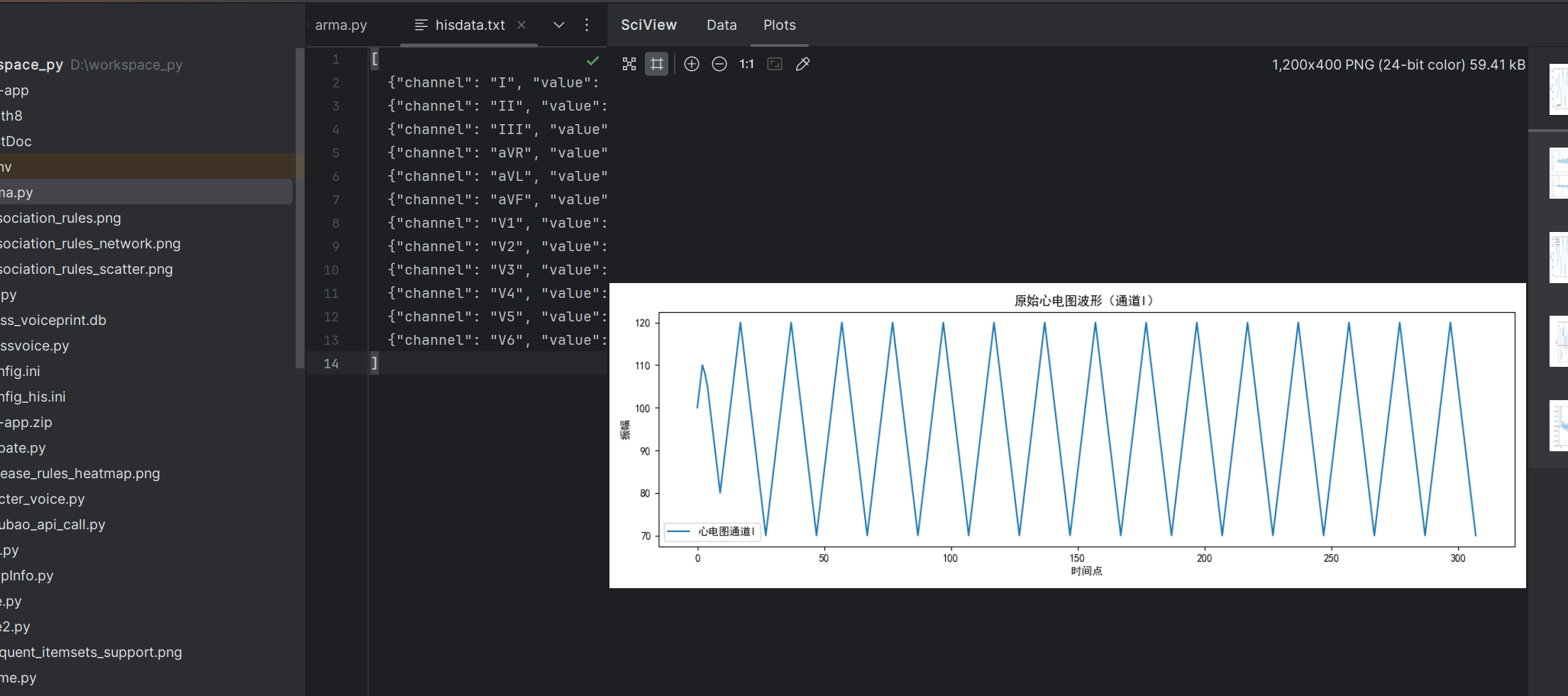
# 绘制原始心电图波形
plt.figure(figsize=(12, 4))
plt.plot(ecg_series.index, ecg_series.values, label=f'心电图通道{ch}')
plt.xlabel('时间点')
plt.ylabel('振幅')
plt.title(f'原始心电图波形(通道{ch})')
plt.legend()
plt.tight_layout()
plt.show()
# 3. 平稳性检验(ADF检验)
def check_stationarity(series):
result = adfuller(series)
print('ADF检验结果:')
print(f'统计量: {result[0]}')
print(f'p值: {result[1]}')
print(f'临界值: {result[4]}')
if result[1] <= 0.05:
print("结论:数据平稳(拒绝原假设)")
return True
else:
print("结论:数据不平稳(接受原假设)")
return False
# 检验平稳性(心电图数据通常近似平稳)
is_stationary = check_stationarity(ecg_series)
# 4. 确定ARMA模型阶数(p, q)
# 绘制ACF和PACF图
fig, (ax1, ax2) = plt.subplots(2, 1, figsize=(12, 8))
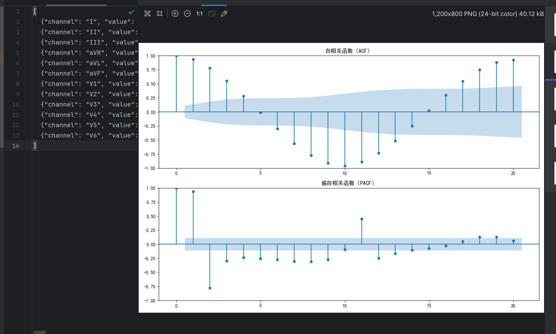
plot_acf(ecg_series, lags=20, ax=ax1) # ACF图用于确定MA阶数q
plot_pacf(ecg_series, lags=20, ax=ax2) # PACF图用于确定AR阶数p
ax1.set_title('自相关函数(ACF)')
ax2.set_title('偏自相关函数(PACF)')
plt.tight_layout()
plt.show()
# 根据ACF和PACF手动选择阶数(示例:p=2, q=1)
p, q = 2, 1 # 可根据图形调整(ACF截尾处为q,PACF截尾处为p)
# 5. 拆分训练集和测试集
train_size = int(len(ecg_series) * 0.8)
train, test = ecg_series[:train_size], ecg_series[train_size:]
print(f"训练集长度:{len(train)},测试集长度:{len(test)}")
# 6. 拟合ARMA模型(ARIMA(p, d=0, q)即ARMA)
model = ARIMA(train, order=(p, 0, q)) # d=0表示不差分(ARMA)
model_fit = model.fit()
print("\n模型拟合结果:")
print(model_fit.summary())
# 7. 模型评估与预测
# 测试集预测
predictions = model_fit.forecast(steps=len(test)) # 预测测试集长度的结果
# 计算MSE评估误差
mse = mean_squared_error(test, predictions)
print(f"\n测试集均方误差(MSE):{mse:.4f}")
# 绘制预测结果与实际值对比
plt.figure(figsize=(12, 4))
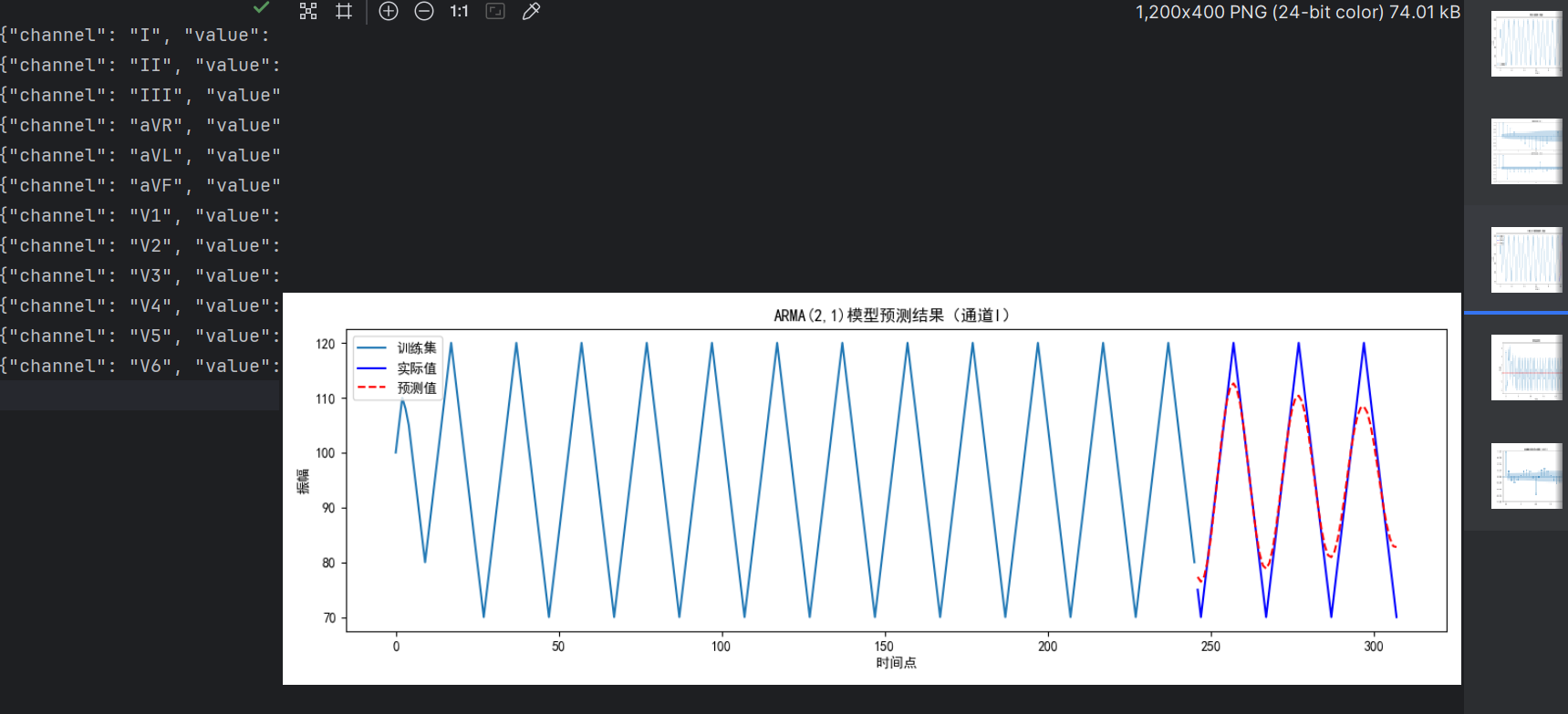
plt.plot(train.index, train.values, label='训练集')
plt.plot(test.index, test.values, label='实际值', color='blue')
plt.plot(test.index, predictions.values, label='预测值', color='red', linestyle='--')
plt.xlabel('时间点')
plt.ylabel('振幅')
plt.title(f'ARMA({p},{q})模型预测结果(通道{ch})')
plt.legend()
plt.tight_layout()
plt.show()
# 8. 残差分析(检验模型是否充分提取信息)
residuals = model_fit.resid
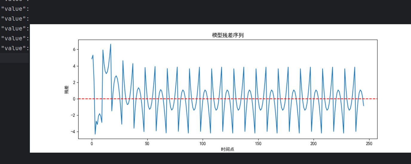
plt.figure(figsize=(12, 4))
plt.plot(residuals)
plt.axhline(y=0, color='r', linestyle='--')
plt.xlabel('时间点')
plt.ylabel('残差')
plt.title('模型残差序列')
plt.show()
# 残差ACF图(应无显著自相关)
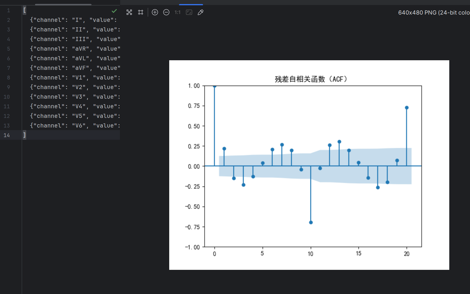
plot_acf(residuals, lags=20)
plt.title('残差自相关函数(ACF)')
plt.show()这段代码是一个完整的心电图(ECG)时间序列分析程序,主要使用 ARMA 模型对心电图数据进行建模和预测。以下是对代码的详细解释:
1. 导入必要的库
|---------------------------------------------------------------------------------------------------------------------------------------------------------------------------------------------------------------------------------------------------------------------------------------------------------|
| import json import numpy as np import pandas as pd import matplotlib.pyplot as plt from statsmodels.tsa.stattools import adfuller, acf, pacf from statsmodels.tsa.arima.model import ARIMA from statsmodels.graphics.tsaplots import plot_acf, plot_pacf from sklearn.metrics import mean_squared_error |
- 数据处理 :json 用于解析 JSON 格式的心电图数据,pandas 和 numpy 用于数据处理和计算。
- 可视化 :matplotlib 用于绘制心电图波形、模型预测结果和残差分析图。
- 时间序列分析 :statsmodels 提供 ADF 检验、ACF/PACF 图和 ARIMA 模型。
- 模型评估 :mean_squared_error 用于计算预测误差。
2. 设置中文字体
|-------------------------------------------------------------------------------------------------------------------------|
| plt.rcParams"font.family" = "SimHei", "Microsoft YaHei" plt.rcParams'axes.unicode_minus' = False # 解决负号显示问题 |
确保中文标题和标签能正常显示,同时修正负号显示问题。
3. 加载并解析心电图数据
|---------------------------------------------------------------------------------------------------------------------------------------------------------------------------------------------------------------------------------------------------------------------------------------------------------------------------------------------------------------------------------------------------------|
| def load_ecg_data(file_path): with open(file_path, 'r', encoding='utf-8') as f: data = json.load(f) ecg_df = pd.DataFrame() for channel in data: ch_name = channel'channel' if len(channel'value') != ecg_df.index.size and not ecg_df.empty: print(f"警告:通道 {ch_name} 的数据长度与其他通道不一致,已跳过。") continue ecg_dfch_name = channel'value' ecg_df = ecg_df.reset_index(drop=True) return ecg_df |
- 功能:从 JSON 文件中读取多通道心电图数据,转换为 DataFrame 格式。
- 数据检查:确保所有通道的数据长度一致,不一致的通道会被跳过(这是之前报错的原因)。
- 返回:包含所有通道数据的 DataFrame,索引重置为连续整数。
4. 数据预处理与可视化
|-----------------------------------------------------------------------------------------------------------------------------------------------------------------------------------------------------------------------------------------------------------------|
| ch = 'I' # 选择分析的通道 ecg_series = ecg_datach.copy() plt.figure(figsize=(12, 4)) plt.plot(ecg_series.index, ecg_series.values, label=f'心电图通道{ch}') plt.xlabel('时间点') plt.ylabel('振幅') plt.title(f'原始心电图波形(通道{ch})') plt.legend() plt.tight_layout() plt.show() |
- 通道选择:默认分析通道 "I"(通常是标准肢体导联)。
- 可视化:绘制原始心电图波形,展示心电信号随时间的变化。
5. 平稳性检验(ADF 检验)
|---------------------------------------------------------------------------------------------------------------------------------------------------------------------------------------------------------------------------------------------------------------------------------------------------------------------------|
| def check_stationarity(series): result = adfuller(series) print('ADF检验结果:') print(f'统计量: {result0}') print(f'p值: {result1}') print(f'临界值: {result4}') if result1 <= 0.05: print("结论:数据平稳(拒绝原假设)") return True else: print("结论:数据不平稳(接受原假设)") return False is_stationary = check_stationarity(ecg_series) |
- 目的:检验时间序列是否平稳(平稳性是 ARMA 模型的前提)。
- 原假设:数据非平稳。若 p 值 ≤ 0.05,则拒绝原假设,认为数据平稳。
- 心电图数据:通常近似平稳,适合 ARMA 建模。
6. 确定 ARMA 模型阶数(p, q)
|-------------------------------------------------------------------------------------------------------------------------------------------------------------------------------------------------------------------------------------------------------------------------------------------------------|
| fig, (ax1, ax2) = plt.subplots(2, 1, figsize=(12, 8)) plot_acf(ecg_series, lags=20, ax=ax1) # ACF图用于确定MA阶数q plot_pacf(ecg_series, lags=20, ax=ax2) # PACF图用于确定AR阶数p ax1.set_title('自相关函数(ACF)') ax2.set_title('偏自相关函数(PACF)') plt.tight_layout() plt.show() p, q = 2, 1 # 可根据图形调整(ACF截尾处为q,PACF截尾处为p) |
- ACF (自相关函数):显示序列与其滞后值之间的相关性,用于确定 MA 阶数(q)。
- PACF (偏自相关函数):显示在去除中间滞后影响后的相关性,用于确定 AR 阶数(p)。
- 阶数选择:根据图形中显著不为零的滞后阶数确定 p 和 q(示例中设为 p=2, q=20)。
7. 拆分训练集和测试集
|------------------------------------------------------------------------------------------------------------------------------------------------------------|
| train_size = int(len(ecg_series) * 0.8) train, test = ecg_series:train_size, ecg_seriestrain_size: print(f"训练集长度:{len(train)},测试集长度:{len(test)}") |
- 划分比例:80% 数据用于训练,20% 用于测试。
- 目的:评估模型在未见过数据上的泛化能力。
8. 拟合 ARMA 模型
|-------------------------------------------------------------------------------------------------------------------------------|
| model = ARIMA(train, order=(p, 0, q)) # d=0表示不差分(ARMA) model_fit = model.fit() print("\n模型拟合结果:") print(model_fit.summary()) |
- 模型定义 :ARIMA(p, d, q) 中,d=0 表示不进行差分,即纯 ARMA 模型。
- 参数解释 :
- AR(p):自回归部分,使用前 p 个时间点的值预测当前值。
- MA(q):移动平均部分,使用前 q 个时间点的误差项修正预测。
- 模型结果:输出 AIC、BIC 等信息,用于评估模型质量。
9. 模型评估与预测
|----------------------------------------------------------------------------------------------------------------------------------------------------------------------------------------------------------------------------------------------------------------------------------------------------------------------------------------------------------------------------------------------------------------------------------------------------------------------------------------|
| predictions = model_fit.forecast(steps=len(test)) mse = mean_squared_error(test, predictions) print(f"\n测试集均方误差(MSE):{mse:.4f}") plt.figure(figsize=(12, 4)) plt.plot(train.index, train.values, label='训练集') plt.plot(test.index, test.values, label='实际值', color='blue') plt.plot(test.index, predictions.values, label='预测值', color='red', linestyle='--') plt.xlabel('时间点') plt.ylabel('振幅') plt.title(f'ARMA({p},{q})模型预测结果(通道{ch})') plt.legend() plt.tight_layout() plt.show() |
- 预测:使用训练好的模型对测试集进行预测。
- 评估指标:MSE(均方误差)衡量预测值与实际值的差异。
- 可视化:对比训练数据、实际值和预测值,直观评估模型效果。
10. 残差分析
|-------------------------------------------------------------------------------------------------------------------------------------------------------------------------------------------------------------------------------------------------------------|
| residuals = model_fit.resid plt.figure(figsize=(12, 4)) plt.plot(residuals) plt.axhline(y=0, color='r', linestyle='--') plt.xlabel('时间点') plt.ylabel('残差') plt.title('模型残差序列') plt.show() plot_acf(residuals, lags=20) plt.title('残差自相关函数(ACF)') plt.show() |
- 残差检查:残差应近似为白噪声(均值为 0,无自相关),否则说明模型未充分提取信息。
- 残差图:观察残差是否随机分布在 0 线附近。
- 残差 ACF 图:检查残差是否存在自相关。若存在显著自相关,需调整模型阶数。
总结
该代码实现了心电图时间序列的完整分析流程:
- 数据加载与预处理:处理多通道 ECG 数据,确保长度一致。
- 可视化:展示原始心电图波形。
- 平稳性检验:使用 ADF 检验确认数据是否适合 ARMA 模型。
- 模型构建:通过 ACF/PACF 图确定阶数,拟合 ARMA 模型。
- 预测与评估:使用 MSE 评估模型性能,可视化预测结果。
- 残差分析:验证模型是否充分提取信息。
通过这个流程,可以对心电图信号进行建模和短期预测,用于心率异常检测或信号滤波等应用。