使用多层神经网络
我们展示如何用TensorFlow构建多层神经网络
###低出生率数据 Low Birthrate data:
#Columns Variable Abbreviation#---------------------------------------------------------------------# Low Birth Weight (0 = Birth Weight >= 2500g, LOW# 1 = Birth Weight < 2500g)# Age of the Mother in Years AGE# Weight in Pounds at the Last Menstrual Period LWT# Race (1 = White, 2 = Black, 3 = Other) RACE# Smoking Status During Pregnancy (1 = Yes, 0 = No) SMOKE# History of Premature Labor (0 = None 1 = One, etc.) PTL# History of Hypertension (1 = Yes, 0 = No) HT# Presence of Uterine Irritability (1 = Yes, 0 = No) UI# Birth Weight in Grams BWT#---------------------------------------------------------------------我们要创建的多层神经网络由三个全链接隐藏层组成, 节点数分别为 50, 25, 和 5
import tensorflow as tf
import matplotlib.pyplot as plt
import csv
import os
import os.path
import random
import numpy as np
import random
import requests
from tensorflow.python.framework import ops
name of data file
birth_weight_file = 'birth_weight.csv'
download data and create data file if file does not exist in current directory
if not os.path.exists(birth_weight_file):
birthdata_url = 'https://github.com/nfmcclure/tensorflow_cookbook/raw/master/01_Introduction/07_Working_with_Data_Sources/birthweight_data/birthweight.dat'
birth_file = requests.get(birthdata_url)
birth_data = birth_file.text.split('\r\n')
birth_header = birth_data0.split('\t')
birth_data = \[float(x) for x in y.split('\\t') if len(x)\>=1 for y in birth_data1: if len(y)>=1]
with open(birth_weight_file, "w") as f:
writer = csv.writer(f)
writer.writerows(birth_header)
writer.writerows(birth_data)
f.close()
read birth weight data into memory
birth_data = \[\]
with open(birth_weight_file, newline='') as csvfile:
csv_reader = csv.reader(csvfile)
birth_header = next(csv_reader)
for row in csv_reader:
birth_data.append(row)
birth_data = \[float(x) for x in row for row in birth_data]
birth_data
Extract y-target (birth weight)
y_vals = np.array(x\[8:9 for x in birth_data])
Filter for features of interest
cols_of_interest = 'AGE', 'LWT', 'RACE', 'SMOKE', 'PTL', 'HT', 'UI'
x_vals = np.array(\[x\[ix for ix, feature in enumerate(birth_header) if feature in cols_of_interest] for x in birth_data])
set batch size for training
batch_size = 10
make results reproducible
seed = 3
np.random.seed(seed)
#tf.set_random_seed(seed)
Split data into train/test = 80%/20%
train_indices = np.random.choice(len(x_vals), round(len(x_vals)*0.8), replace=False)
test_indices = np.array(list(set(range(len(x_vals))) - set(train_indices)))
x_vals_train = x_valstrain_indices
x_vals_test = x_valstest_indices
y_vals_train = y_valstrain_indices
y_vals_test = y_valstest_indices
Record training column max and min for scaling of non-training data
train_max = np.max(x_vals_train, axis=0)
train_min = np.min(x_vals_train, axis=0)
Normalize by column (min-max norm to be between 0 and 1)
def normalize_cols(mat, max_vals, min_vals):
return (mat - min_vals) / (max_vals - min_vals)
x_vals_train = np.nan_to_num(normalize_cols(x_vals_train, train_max, train_min))
x_vals_test = np.nan_to_num(normalize_cols(x_vals_test, train_max, train_min))
#定义权重和偏置。
Define Variable Functions (weights and bias)
def init_weight(shape, st_dev):
weight = tf.Variable(tf.random.normal(shape, stddev=st_dev))
return(weight)
def init_bias(shape, st_dev):
bias = tf.Variable(tf.random.normal(shape, stddev=st_dev))
return(bias)
#定义模型!我们先创建一个根据变量生成全链接层的函数。
x_data = tf.Variable(np.random.randn(1,7),dtype=tf.float32)
y_target = tf.Variable(np.random.randn(1,1),dtype=tf.float32)
Create a fully connected layer:
def fully_connected(input_layer, weights, biases):
layer = tf.add(tf.matmul(input_layer, weights), biases)
return(tf.nn.relu(layer))
#我们初始化变量并开始训练循环。
learning_rate=0.001
Training loop
loss_vec = \[\]
test_loss = \[\]
weight_1 = init_weight(shape=7, 25, st_dev=1.0)
bias_1 = init_bias(shape=25, st_dev=10.0)
weight_2 = init_weight(shape=25, 10, st_dev=1.0)
bias_2 = init_bias(shape=10, st_dev=10.0)
weight_3 = init_weight(shape=10, 3, st_dev=1.0)
bias_3 = init_bias(shape=3, st_dev=10.0)
weight_4 = init_weight(shape=3, 1, st_dev=1.0)
bias_4 = init_bias(shape=1, st_dev=1.0)
for i in range(3000):
rand_index = np.random.choice(len(x_vals_train), size=batch_size)
rand_x = x_vals_trainrand_index
rand_y = np.transpose(y_vals_train\[rand_index])
with tf.GradientTape() as tape:
#--------Create the first layer (50 hidden nodes)--------
layer_1 = fully_connected(x_data, weight_1, bias_1)
#--------Create second layer (25 hidden nodes)--------
layer_2 = fully_connected(layer_1, weight_2, bias_2)
#--------Create third layer (5 hidden nodes)--------
layer_3 = fully_connected(layer_2, weight_3, bias_3)
#--------Create output layer (1 output value)--------
final_output = fully_connected(layer_3, weight_4, bias_4)
Declare loss function (L1)
loss = tf.reduce_mean(tf.abs(y_target - final_output))
grads=tape.gradient(loss,weight_1,bias_1,weight_2,bias_2,weight_3,bias_3,weight_4,bias_4)
loss_vec.append(loss)
weight_1.assign_sub(learning_rate*grads0)
bias_1.assign_sub(learning_rate*grads1)
weight_2.assign_sub(learning_rate*grads2)
bias_2.assign_sub(learning_rate*grads3)
weight_3.assign_sub(learning_rate*grads4)
bias_3.assign_sub(learning_rate*grads5)
weight_4.assign_sub(learning_rate*grads6)
bias_4.assign_sub(learning_rate*grads7)
#test_loss.append(test_temp_loss)
if (i+1) % 25 == 0:
print('Generation: ' + str(i+1) + '. Loss = ' + str(loss.numpy()))
#绘制损失函数。
%matplotlib inline
Plot loss (MSE) over time
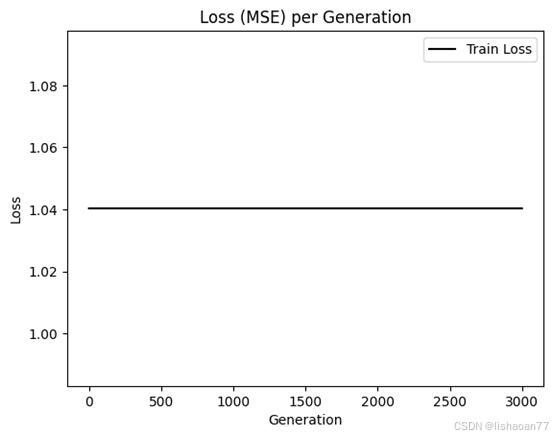
plt.plot(loss_vec, 'k-', label='Train Loss')
#plt.plot(test_loss, 'r--', label='Test Loss')
plt.title('Loss (MSE) per Generation')
plt.legend(loc='upper right')
plt.xlabel('Generation')
plt.ylabel('Loss')
plt.show()
Create variable definition
def init_variable(shape):
return(tf.Variable(tf.random.normal(shape=shape)))
Create a logistic layer definition
def logistic(input_layer, multiplication_weight, bias_weight, activation = True):
linear_layer = tf.add(tf.matmul(input_layer, multiplication_weight), bias_weight)
We separate the activation at the end because the loss function will
implement the last sigmoid necessary
if activation:
return(tf.nn.sigmoid(linear_layer))
else:
return(linear_layer)
Declare optimizer
#my_opt = tf.train.AdamOptimizer(learning_rate = 0.002)
#train_step = my_opt.minimize(loss)
Actual Prediction
A1 = init_variable(shape=7,14)
b1 = init_variable(shape=14)
A2 = init_variable(shape=14,5)
b2 = init_variable(shape=5)
A3 = init_variable(shape=5,1)
b3 = init_variable(shape=1)
optimizer = tf.optimizers.SGD(learning_rate)
Training loop
loss_vec = \[\]
train_acc = \[\]
test_acc = \[\]
for i in range(3000):
rand_index = np.random.choice(len(x_vals_train), size=batch_size)
rand_x = x_vals_trainrand_index
rand_y = np.transpose(y_vals_train\[rand_index])
with tf.GradientTape() as tape:
First logistic layer (7 inputs to 14 hidden nodes)
logistic_layer1 = logistic(x_data, A1, b1)
Second logistic layer (14 hidden inputs to 5 hidden nodes)
logistic_layer2 = logistic(logistic_layer1, A2, b2)
Final output layer (5 hidden nodes to 1 output)
final_output = logistic(logistic_layer2, A3, b3, activation=False)
Declare loss function (Cross Entropy loss)
loss = tf.reduce_mean(tf.nn.sigmoid_cross_entropy_with_logits(logits=final_output, labels=y_target))
grads=tape.gradient(loss,A1,b1,A2,b2,A3,b3)
optimizer.apply_gradients(zip(grads, A1,b1,A2,b2,A3,b3))
loss_vec.append(loss)
#A1.assign_sub(learning_rate*grads0)
#b1.assign_sub(learning_rate*grads1)
#A2.assign_sub(learning_rate*grads2)
#b2.assign_sub(learning_rate*grads3)
#A3.assign_sub(learning_rate*grads4)
#b3.assign_sub(learning_rate*grads5)
if (i+1)%150==0:
print('Loss = ' + str(loss.numpy()))
%matplotlib inline
Plot loss over time
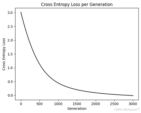
plt.plot(loss_vec, 'k-')
plt.title('Cross Entropy Loss per Generation')
plt.xlabel('Generation')
plt.ylabel('Cross Entropy Loss')
plt.show()