《Build a Large Language Model (From Scratch)》是一本畅销的深入浅出介绍大语言模型理论知识和工程实践的书。作者在消费级的个人电脑上,逐步实现大语言模型的数据处理、模型构建、预训练和微调。《LLMs from scratch》是该书的官方代码仓库,包含大语言模型的数据处理、模型构建、预训练和微调的相关代码。《从零构建大模型》是《Build a Large Language Model (From Scratch)》的中译版本。本文是笔者阅读《从零构建大模型》的阅读笔记,记录书中涉及的大语言模型的数据处理、模型构建和预训练的理论知识以及笔者在个人电脑上进行工程实践的相关代码和运行结果。文中如有不足之处,欢迎指正。
环境准备
笔者个人电脑品牌型号为MacBook Pro,芯片为Apple M4 Pro,内存为24G,操作系统为Sequoia 15.5,且已安装Git(版本为2.39.5)、Python 3(版本为3.9.6)和UV(版本为0.7.14)。
下载《从零构建大模型》的代码:
shell
git clone --depth 1 https://github.com/rasbt/LLMs-from-scratch.git进入代码目录,按照其中"setup/01_optional-python-setup-preferences/README.md"的说明进行环境准备。
创建环境:
shell
uv venv --python=python3.10激活环境:
shell
source .venv/bin/activate安装依赖:
shell
uv pip install -r requirements.txt检查环境:
shell
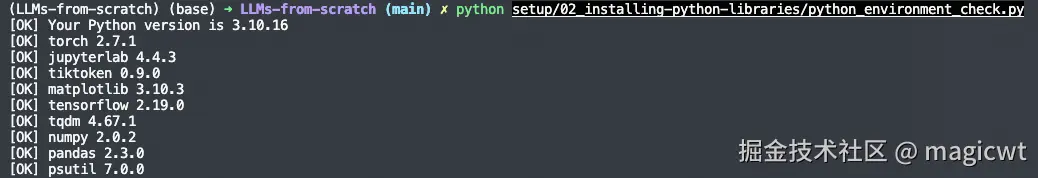
python setup/02_installing-python-libraries/python_environment_check.py执行上述脚本,检查requirements.txt中要求的依赖是否已安装。requirements.txt的内容如下所示:
plain
torch >= 2.3.0             # all
jupyterlab >= 4.0          # all
tiktoken >= 0.5.1          # ch02; ch04; ch05
matplotlib >= 3.7.1        # ch04; ch06; ch07
tensorflow >= 2.18.0       # ch05; ch06; ch07
tqdm >= 4.66.1             # ch05; ch07
numpy >= 1.26, < 2.1       # dependency of several other libraries like torch and pandas
pandas >= 2.2.1            # ch06
psutil >= 5.9.5            # ch07; already installed automatically as dependency of torch
执行脚本后的输出如图1所示,依赖已安装。
启动JupyterLab:
shell
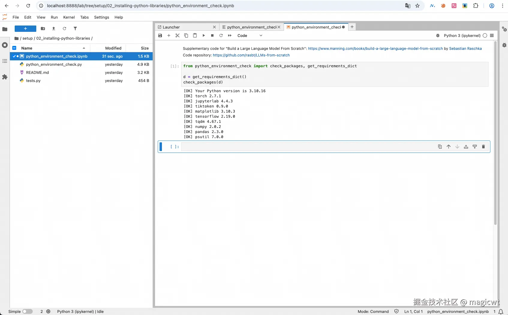
jupyter lab启动后,浏览器输入"http://localhost:8888/lab ",打开JupyterLab,可以浏览代码,如图2所示。

也可以运行代码,如图3所示。
处理文本数据
理解词嵌入
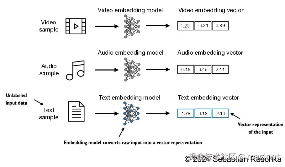
视频、音频、文本,这些不同类型的输入,可以通过各个类型所对应的嵌入模型(embedding model)转化为嵌入向量(embedding vector),如图4所示。
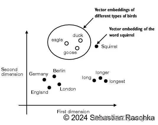
语义相似的文本的嵌入向量在向量空间中距离相近,如图5所示,eagle、duck、goose这三个文本语义相似,同属鸟类,因此它们的嵌入向量在向量空间中距离相近,在一个类簇中。
文本分词
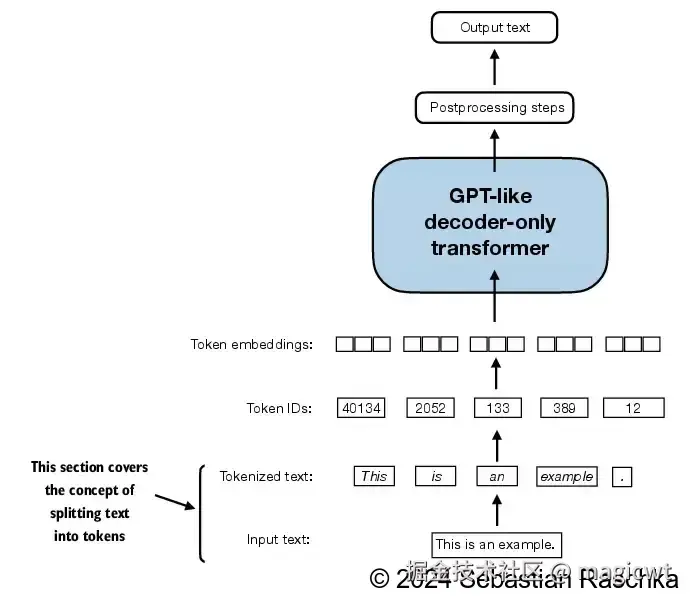
对文本进行分词,划分为多个词元(Token),即将文本转化为词元序列。书中使用Edith Wharton的短篇小说------《The Verdict》作为预训练大语言模型的文本数据集。代码中也包含了该小说的全文,文件地址是"ch02/01_main-chapter-code/the-verdict.txt"。图6是一个示例,将"This is an example."划分为"This"、"is"、"an"、"example"、"."这些词元。另外,一般还会引入一些特殊的词元来增强对文本的表示,例如,可以使用"<|endoftext|>"来表示文本的末尾。
将词元转化为词元ID
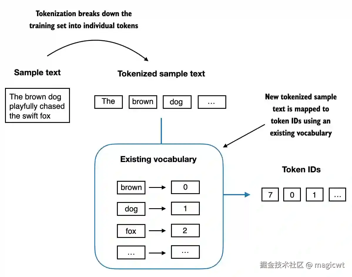
使用词典存储所有的词元,词典中的每个词元均有对应的唯一ID。将文本转化为词元序列后,再通过查询词典,得到每个词元所对应的ID,将词元序列进一步转化为词元ID序列,如图7所示。
BPE
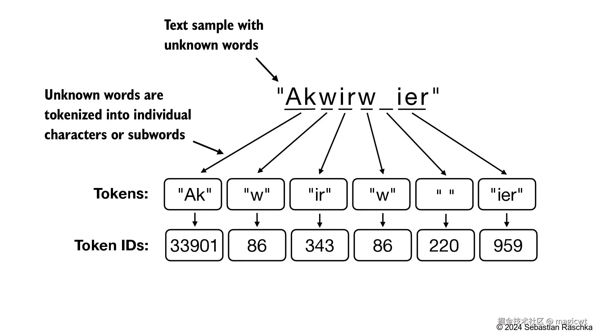
前序介绍中的分词方法基于空格,将文本划分为多个单词。GPT-2实际使用字节对编码(BPE)作为其分词器。该方法可以将词典中未包含的单词拆解为更小的子词单元甚至单个字符,从而有效处理词典外的单词。 例如,若GPT-2的词典中没有"unfamiliarword"这个词,则BPE可能会将这个词切分为"unfam"、"iliar"、"word" 这三个子词的组合或其他子词组合。图8是另一个例子,若GPT-2的词典中没有"Akwirw"这个词,则BPE将这个词切分为"Ak"、"w"、"ir"、"w"这四个子词的组合。
原始BPE分词器代码可在OpenAI的GPT-2项目中找到,地址如下:github.com/openai/gpt-... 。书中采用OpenAI开源的tiktoken库实现的BPE分词器,该库通过Rust语言重写核心算法以提升计算性能。使用BPE分词器对测试文本进行分词,编码为词元ID序列,再解码词元ID序列,还原文本的代码如下所示:
python
import importlib
import tiktoken

# 初始化BPE分词器
tokenizer = tiktoken.get_encoding("gpt2")

# 测试文本
text = (
    "Hello, do you like tea? <|endoftext|> In the sunlit terraces"
    "of someunknownPlace."
)

# 编码
# 将文本编码为词元ID序列
integers = tokenizer.encode(text, allowed_special={"<|endoftext|>"})
print("将文本编码为词元ID序列: ", integers)

# 解码
# 将词元ID序列解码为文本
strings = tokenizer.decode(integers)
print("将词元ID序列解码为文本: ", strings)
代码执行结果如下所示:
plain
将文本编码为词元ID序列:  [15496, 11, 466, 345, 588, 8887, 30, 220, 50256, 554, 262, 4252, 18250, 8812, 2114, 1659, 617, 34680, 27271, 13]
将词元ID序列解码为文本:  Hello, do you like tea? <|endoftext|> In the sunlit terracesof someunknownPlace.
使用BPE分词器对《The Verdict》进行分词,编码为词元ID序列的代码如下所示:
python
with open("the-verdict.txt", "r", encoding="utf-8") as f:
    raw_text = f.read()

enc_text = tokenizer.encode(raw_text)
print("小说词元ID序列长度: ", len(enc_text))
print("小说词元ID序列前100个词元: ", enc_text[:100])
print("小说词元ID序列后100个词元: ",enc_text[-100:])
代码执行结果如下所示:
plain
小说词元ID序列长度:  5145
小说词元ID序列前100个词元:  [40, 367, 2885, 1464, 1807, 3619, 402, 271, 10899, 2138, 257, 7026, 15632, 438, 2016, 257, 922, 5891, 1576, 438, 568, 340, 373, 645, 1049, 5975, 284, 502, 284, 3285, 326, 11, 287, 262, 6001, 286, 465, 13476, 11, 339, 550, 5710, 465, 12036, 11, 6405, 257, 5527, 27075, 11, 290, 4920, 2241, 287, 257, 4489, 64, 319, 262, 34686, 41976, 13, 357, 10915, 314, 2138, 1807, 340, 561, 423, 587, 10598, 393, 28537, 2014, 198, 198, 1, 464, 6001, 286, 465, 13476, 1, 438, 5562, 373, 644, 262, 1466, 1444, 340, 13, 314, 460, 3285, 9074, 13, 46606, 536]
小说词元ID序列后100个词元:  [257, 1808, 314, 1234, 2063, 12, 1326, 3147, 1146, 438, 1, 44140, 757, 1701, 339, 30050, 503, 13, 366, 2215, 262, 530, 1517, 326, 6774, 502, 6609, 1474, 683, 318, 326, 314, 2993, 1576, 284, 2666, 572, 1701, 198, 198, 1544, 6204, 510, 290, 8104, 465, 1021, 319, 616, 8163, 351, 257, 6487, 13, 366, 10049, 262, 21296, 286, 340, 318, 326, 314, 4808, 321, 62, 991, 12036, 438, 20777, 41379, 293, 338, 1804, 340, 329, 502, 0, 383, 520, 5493, 82, 1302, 3436, 11, 290, 1645, 1752, 438, 4360, 612, 338, 645, 42393, 803, 674, 1611, 286, 1242, 526]
创建词元嵌入
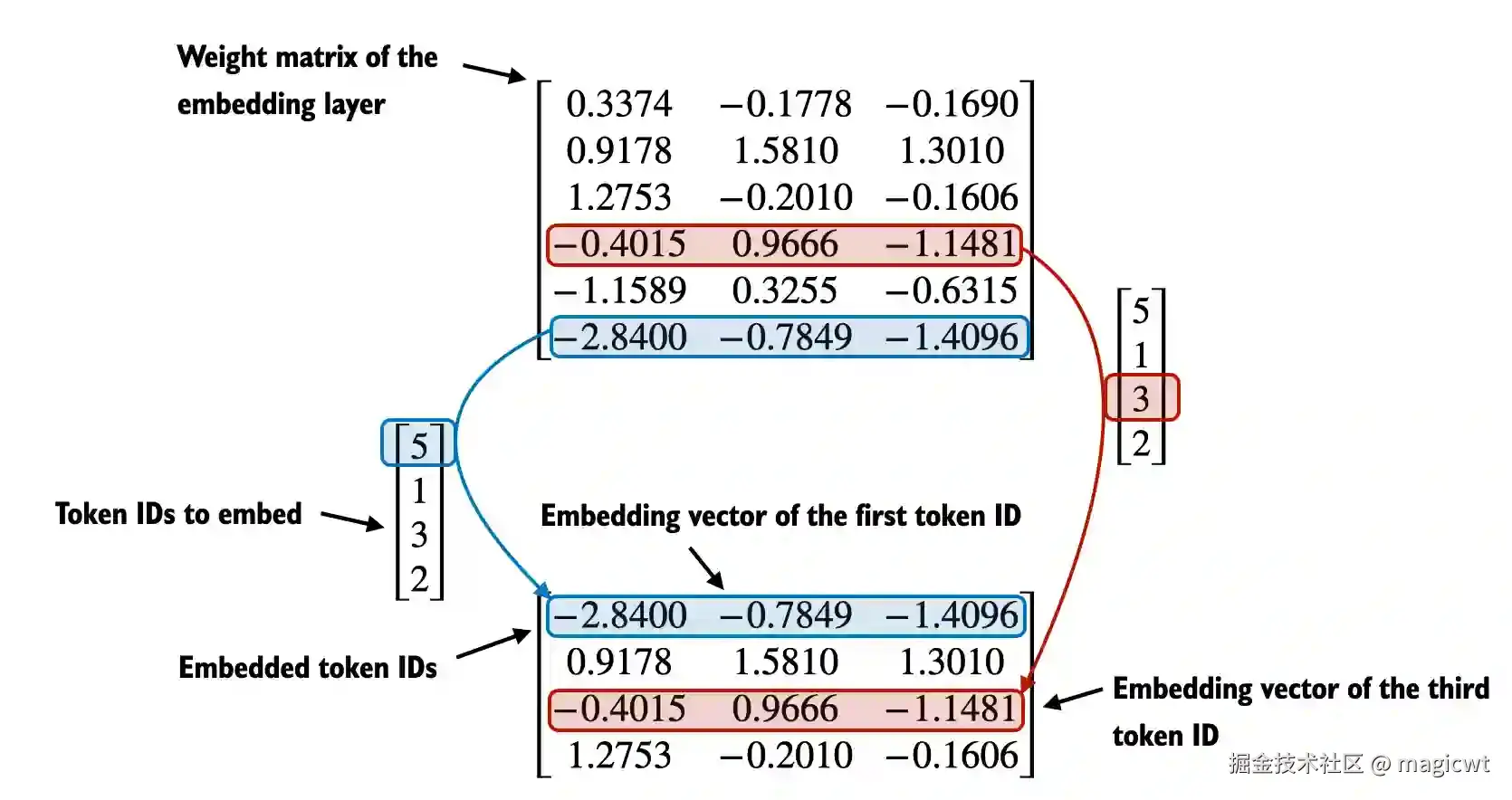
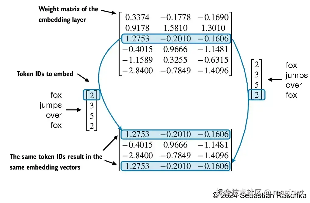
进一步将词元ID序列转化为词元向量序列,该操作通过一个Embedding层完成,Embedding层就是一个可学习的权重矩阵,该矩阵的行数是词元词典的大小,该矩阵的列数是词元向量的维度。矩阵的每一行表示该行号所对应的词元ID的词元向量,例如词元ID为3的词元向量即矩阵的第4行(行号从0开始,第4行的行号是3)-------0.4015, 0.9666, -1.1481,如图9所示。
定义Embedding层的代码如下所示,该Embedding层的行数为50257,即词典的大小为50257,该Embedding层的列数为256,即词元向量的维度为256:
python
vocab_size = 50257
output_dim = 256

token_embedding_layer = torch.nn.Embedding(vocab_size, output_dim)
编码位置信息
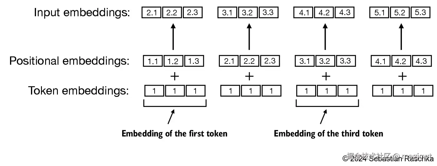
如果同一个词元在词元序列中出现多次,其在序列中不同的位置表达的语义可能有所不同,但通过上面的Embedding层后,同一个词元在词元序列中的不同位置均会转化为相同的词元向量,如图10所示。
因此,对于词元序列中的每个词元,其在Embedding层输出的原始向量基础上,还会叠加位置向量,从而使得同一个词元在词元序列中的不同位置的向量有所不同,如图11所示。
注意力机制
长序列建模的问题
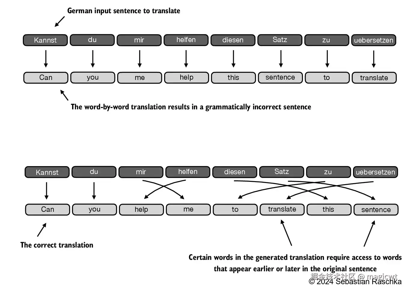
考虑翻译问题,由于源语言和目标语言的语法结构不同,无法简单地逐个单词进行翻译。生成翻译时,一些词语需要参考在原句中较早或较晚出现的词,如图12所示。为了处理这个问题,通常使用一个包含编码器和解码器两个子模块的深度神经网络。编码器首先读取和处理整个文本,解码器则负责生成翻译后的文本。
在 Transformer 出现之前,循环神经网络(recurrent neural network,RNN)是语言翻译中最流行的编码器-解码器架构。
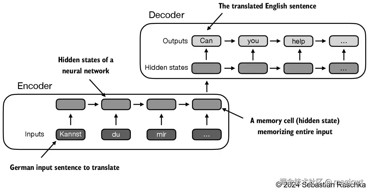
在RNN中,输入文本被传递给编码器以逐步处理。编码器在每一步都会更新其隐状态(隐藏层的内部值),试图在最终的隐状态中捕捉输入句子的全部含义,如图13所示。然后,解码器使用这个最终的隐状态开始逐字生成翻译后的句子。解码器同样在每一步更新其隐状态,该状态应包含为下一单词预测所需的上下文信息。
RNN的一个主要限制是,在解码阶段,RNN 无法直接访问编码器中的早期隐状态。因此,它只能依赖当前的隐状态,这个状态包含了所有相关信息。这可能导致上下文丢失,特别是在复杂句子中,依赖关系可能跨越较长的距离。
自注意力是Transformer模型中的一种机制,它通过允许一个序列中的每个位置与同一序列中的其他所有位置进行交互并权衡其重要性,来计算出更高效的输入表示,从而解决RNN只能依赖当前隐状态的问题。
Transformer最早在《Attention is all you need》中被提出。《Attention Is All You Need》是Google于2017年发表的一篇经典论文,其开创性的设计了Transformer模型结构,对于序列问题,通过编码器输出隐向量序列,再通过解码器输出目标序列,模型引入了注意力机制,充分挖掘序列各节点之间的深度信息,并通过矩阵计算的并行化加速模型训练和推理性能。关于Transformer的详细介绍,可以阅读论文原文或笔者梳理的《AIGC系列-Transformer论文阅读笔记》。
通过自注意力机制关注输入的不同部分
首先实现一个不包含任何可训练权重的简化的自注意力机制变体,如图14所示。目标是在引入可训练权重之前,阐明自注意力中的一些关键概念。
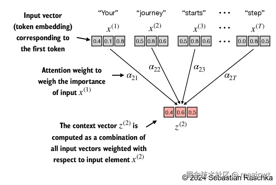
图14显示了一个输入序列,记为 x,它由 T个元素组成,分别表示为 x(1)到 x(T)。这个序列通常代表文本(如一个句子),并且该文本已经被转换为词元嵌入。
例如,考虑输入文本为"Your journey starts with one step."。在这种情况下,文本序列中的每个元素(如第一个词元 x(1))都对应一个 d维的嵌入向量,该向量代表了一个特定的词元,比如"Your"。在图中,这些输入向量被表示为三维嵌入。
在自注意力机制中,我们的目标是为输入序列中的每个元素 x(i)计算上下文向量 z(i)。上下文向量(context vector)可以被理解为一种包含了序列中所有元素信息的嵌入向量。
为了说明这个概念,我们重点关注第二个输入元素 x(2)(对应于词元"journey")的嵌入向量及其对应的上下文向量 z(2),如图14底部所示。这个增强的上下文向量 z(2)是一个嵌入,包含了关于 x(2)及其他所有输入元素( x(1) 到 x(T))的信息。
上下文向量在自注意力机制中起着关键作用。它们的目的是通过结合序列中其他所有元素的信息,为输入序列(如一个句子)中的每个元素创建丰富表示,如图14所示。这在大语言模型中至关重要,因为这些模型需要理解句子中单词之间的关系和相关性。
图14中, z(2)可表示为:
z(2)=i=1∑Tα2i⋅x(i)
其中, α2i表示 x(i)对 x(T)的注意力权重。
而对于所有 T个元素的上下文向量:
z=W⋅x
其中, z= z(1)z(2)⋯z(T) , W为注意力权重矩阵,第 i行第 j列为 αij, x= x(1)x(2)⋯x(T) 。
实现带可训练权重的自注意力机制
而在Transformer中,注意力权重是可以学习的。通过引入3个可训练的参数矩阵 Wq、 Wk和 Wv,将输入词元 x(i)分别映射为查询向量 q(i)、键向量 k(i)和值向量 v(i):
q=Wq⋅x
k=Wk⋅x
v=Wv⋅x
其中, q= q(1)q(2)⋯q(T) , k= k(1)k(2)⋯k(T) , v= v(1)v(2)⋯v(T) 。
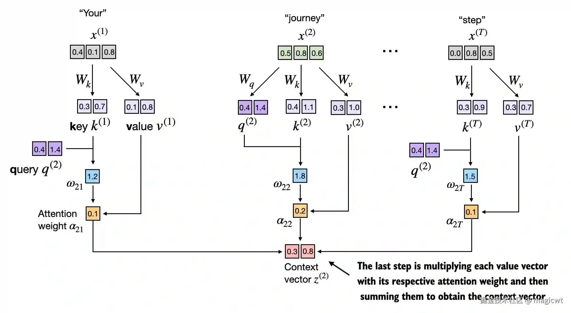
仍是以 z(2)为例,如图15所示,先通过查询向量和键向量点积得到注意力得分,即
w2i=q(2)⋅k(i)
再通过Softmax函数对注意力得分进行归一化得到注意力权重,注意这里在对注意力得分进行归一化之前会先除以维度的平方根进行缩放,避免梯度过小,从而提升训练性能,这一技巧源自Transformer的论文,也是缩放点积注意力中"缩放点积"的由来:
α2i=∑j=1Tew2j/d ew2i/d
对值向量按注意力权重进行加权求和得到上下文向量:
z(2)=i=1∑Tα2i⋅x(i)
带可训练权重的自注意力机制的代码如下所示:
python
import torch
import torch.nn as nn

# 自注意力实现(v1)
class SelfAttention_v1(nn.Module):

    def __init__(self, d_in, d_out):
        super().__init__()
        # 初始化查询参数矩阵
        self.W_query = nn.Parameter(torch.rand(d_in, d_out))
        # 初始化键参数矩阵
        self.W_key   = nn.Parameter(torch.rand(d_in, d_out))
        # 初始话值参数矩阵
        self.W_value = nn.Parameter(torch.rand(d_in, d_out))

    def forward(self, x):
        # 键向量
        keys = x @ self.W_key
        # 查询向量
        queries = x @ self.W_query
        # 值向量
        values = x @ self.W_value

        # 查询向量和键向量点积得到注意力得分
        attn_scores = queries @ keys.T # omega
        # 通过Softmax函数对注意力得分进行归一化得到注意力权重
        # 注意这里在对注意力得分进行归一化之前会先除以维度的平方根进行缩放,避免梯度过小,从而提升训练性能,这一技巧源自Transformer的论文,也是缩放点积注意力中"缩放点积"的由来
        attn_weights = torch.softmax(
            attn_scores / keys.shape[-1]**0.5, dim=-1
        )

        # 对值向量按注意力权重进行加权求和得到上下文向量
        context_vec = attn_weights @ values
        return context_vec

torch.manual_seed(123)
# 模拟文本"Your journey starts with one step"的词元向量序列
inputs = torch.tensor(
  [[0.43, 0.15, 0.89], # Your     (x^1)
   [0.55, 0.87, 0.66], # journey  (x^2)
   [0.57, 0.85, 0.64], # starts   (x^3)
   [0.22, 0.58, 0.33], # with     (x^4)
   [0.77, 0.25, 0.10], # one      (x^5)
   [0.05, 0.80, 0.55]] # step     (x^6)
)
# 词元向量维度为3
d_in = inputs.shape[1] # the input embedding size, d=3
# 上下文向量维度为2
d_out = 2 # the output embedding size, d=2
# 输出经过自注意力层后的上下文向量,长度和输入的词元向量序列长度一致,为6
sa_v1 = SelfAttention_v1(d_in, d_out)
print(sa_v1(inputs))
代码执行结果如下所示,输出经过自注意力层后的上下文向量,长度和输入的词元向量序列长度一致,为6,其中每一个为对应位置的输入词元的上下文向量,而每个上下文向量的维度为2。
plain
tensor([[0.2996, 0.8053],
        [0.3061, 0.8210],
        [0.3058, 0.8203],
        [0.2948, 0.7939],
        [0.2927, 0.7891],
        [0.2990, 0.8040]], grad_fn=<MmBackward0>)
采用线性层替代参数矩阵,若线性层无偏置,则等价于参数矩阵。相比手动实现 nn.Parameter(torch.rand(...)),使用nn.Linear的一个重要优势是它提供了优化的权重初始化方案,从而有助于模型训练的稳定性和有效性。修改后的带可训练权重的自注意力机制的代码如下所示:
python
import torch
import torch.nn as nn

# 自注意力实现(v2)
class SelfAttention_v2(nn.Module):

    def __init__(self, d_in, d_out, qkv_bias=False):
        super().__init__()
        # 采用线性层替代参数矩阵,若线性层无偏置,则等价于参数矩阵
        self.W_query = nn.Linear(d_in, d_out, bias=qkv_bias)
        self.W_key   = nn.Linear(d_in, d_out, bias=qkv_bias)
        self.W_value = nn.Linear(d_in, d_out, bias=qkv_bias)

    def forward(self, x):
        keys = self.W_key(x)
        queries = self.W_query(x)
        values = self.W_value(x)

        attn_scores = queries @ keys.T
        attn_weights = torch.softmax(attn_scores / keys.shape[-1]**0.5, dim=-1)

        context_vec = attn_weights @ values
        return context_vec

torch.manual_seed(789)
# 模拟文本"Your journey starts with one step"的词元向量序列
inputs = torch.tensor(
    [[0.43, 0.15, 0.89], # Your     (x^1)
     [0.55, 0.87, 0.66], # journey  (x^2)
     [0.57, 0.85, 0.64], # starts   (x^3)
     [0.22, 0.58, 0.33], # with     (x^4)
     [0.77, 0.25, 0.10], # one      (x^5)
     [0.05, 0.80, 0.55]] # step     (x^6)
)
# 词元向量维度为3
d_in = inputs.shape[1] # the input embedding size, d=3
# 上下文向量维度为2
d_out = 2 # the output embedding size, d=2
# 输出经过自注意力层后的上下文向量,长度和输入的词元向量序列长度一致,为6
sa_v2 = SelfAttention_v2(d_in, d_out)
print(sa_v2(inputs))
代码执行结果如下所示,输出仍是经过自注意力层后的上下文向量,长度和输入的词元向量序列长度一致,为6:
plain
tensor([[-0.0739,  0.0713],
        [-0.0748,  0.0703],
        [-0.0749,  0.0702],
        [-0.0760,  0.0685],
        [-0.0763,  0.0679],
        [-0.0754,  0.0693]], grad_fn=<MmBackward0>)
利用因果注意力隐藏未来词汇
改进自注意力机制,引入因果机制和多头机制。因果机制的作用是调整注意力机制,防止模型访问序列中未来的信息,这在语言建模等任务中尤为重要,因为每个词的预测只能依赖之前出现的词。
因果注意力(也称为掩码注意力)是一种特殊的自注意力形式。它限制模型在处理任何给定词元时,只能基于序列中的先前和当前输入来计算注意力分数,而标准的自注意力机制可以一次性访问整个输入序列。
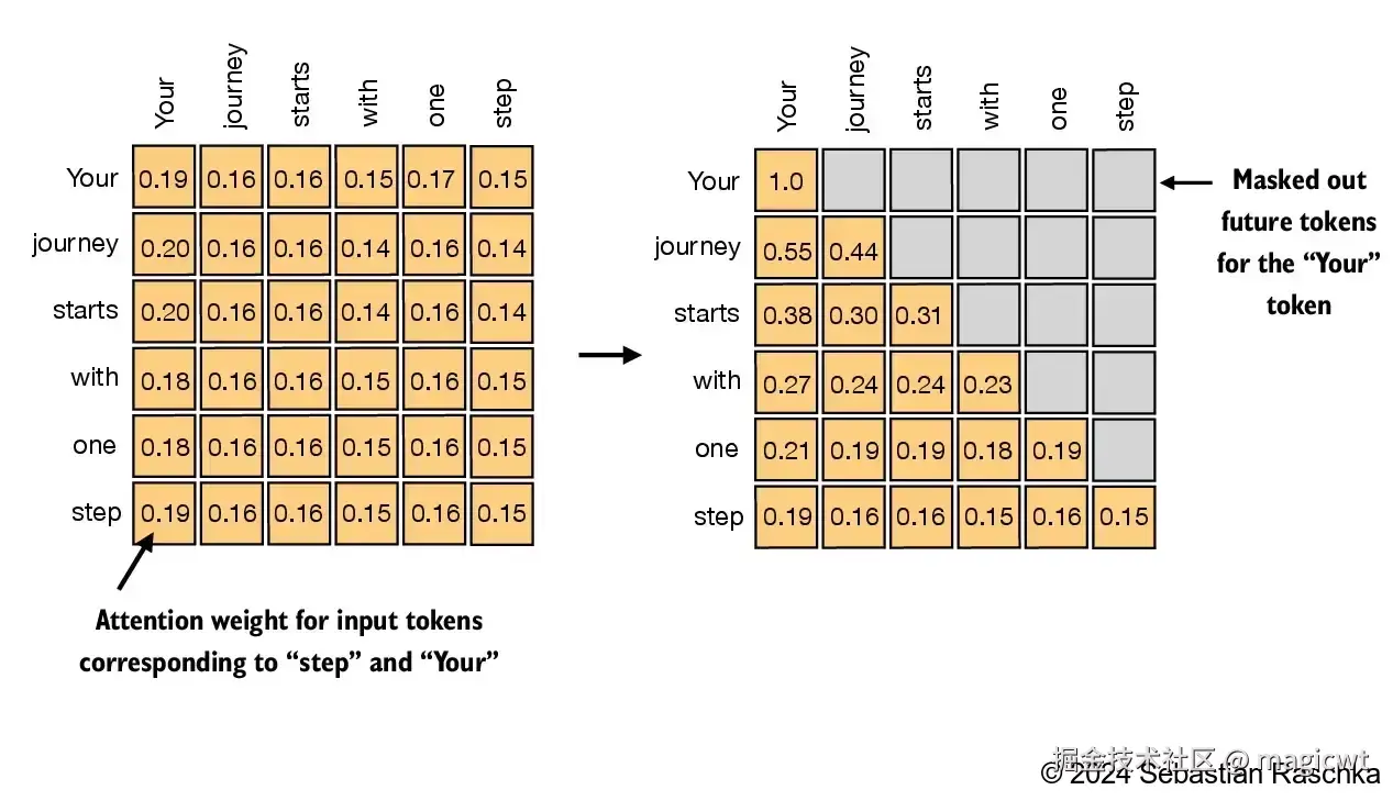
通过修改标准自注意力机制来创建因果注意力机制,这是在后续章节中开发大语言模型的关键步骤。对于每个处理的词元,需要掩码当前词元之后的后续词元,如图16右侧所示,掩码对角线以上的注意力权重,并归一化未掩码的注意力权重,使得每一行的权重之和为 1。
图16左侧是未掩码的注意力权重示意,第 i行表示序列中各词元对第 i个词元的注意力权重,第 i行第 j列表示序列中第 j个词元对第 i个词元的注意力权重,例如,第2行表示序列中各词元对第2个词元(journey)的注意力权重,分别是0.20、0.16、0.16、0.14、0.16、0.14。
图16右侧是掩码并在掩码后重新归一化的注意力权重示意,第2行表示的"journey"只可见其前面的"Your"和其自身,不可见其后面的"starts"、"with"、"one"、"step",因此,序列中只有"Your"和"journey"对"journey"有注意力权重,分别是0.55和0.44。
因果注意力中,注意力权重矩阵的右上角权重均为0,而注意力权重是通过Softmax函数对注意力得分进行归一化得到,而对于Softmax函数,若注意力得分为负无穷大,则其注意力权重趋近为0,因此,可以通过将自注意力的注意力得分矩阵的右上角全置为负无穷大来实现因果注意力。
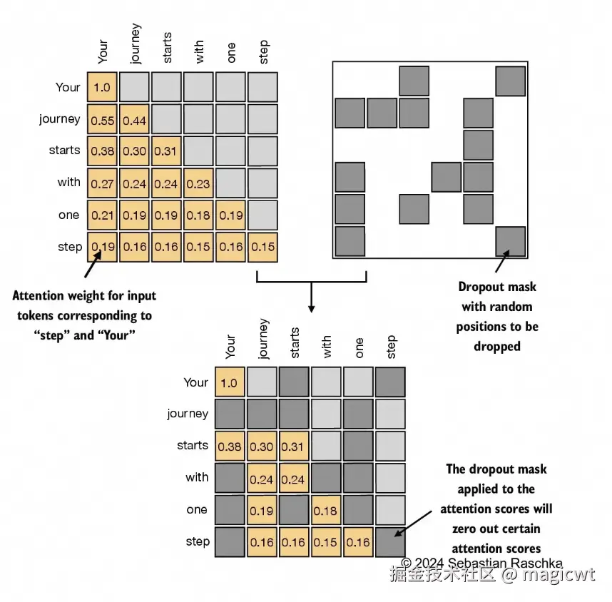
dropout是深度学习中的一种技术,通过在训练过程中随机忽略一些隐藏层单元来有效地"丢弃"它们。这种方法有助于减少模型对特定隐藏层单元的依赖,从而避免过拟合。需要强调的是,dropout仅在训练期间使用,训练结束后会被取消。在Transformer架构中,通常会在两个特定时间点使用dropout:一是计算注意力权重之后,二是将这些权重应用于值向量之后。在计算注意力权重之后应用dropout掩码的示意如图17所示。
带有dropout的因果注意力实现如下:
python
import torch
import torch.nn as nn

# 带掩码的因果注意力实现
class CausalAttention(nn.Module):

    def __init__(self, d_in, d_out, context_length,
                 dropout, qkv_bias=False):
        super().__init__()
        self.d_out = d_out
        self.W_query = nn.Linear(d_in, d_out, bias=qkv_bias)
        self.W_key   = nn.Linear(d_in, d_out, bias=qkv_bias)
        self.W_value = nn.Linear(d_in, d_out, bias=qkv_bias)
        self.dropout = nn.Dropout(dropout) # New
        self.register_buffer('mask', torch.triu(torch.ones(context_length, context_length), diagonal=1)) # New

    def forward(self, x):
        b, num_tokens, d_in = x.shape # New batch dimension b
        # For inputs where `num_tokens` exceeds `context_length`, this will result in errors
        # in the mask creation further below.
        # In practice, this is not a problem since the LLM (chapters 4-7) ensures that inputs
        # do not exceed `context_length` before reaching this forward method.
        keys = self.W_key(x)
        queries = self.W_query(x)
        values = self.W_value(x)

        attn_scores = queries @ keys.transpose(1, 2) # Changed transpose
        # 以上计算注意力得分和自注意力实现中的逻辑一致
        # 将注意力得分矩阵的右上角置为负无穷大
        attn_scores.masked_fill_(  # New, _ ops are in-place
            self.mask.bool()[:num_tokens, :num_tokens], -torch.inf)  # `:num_tokens` to account for cases where the number of tokens in the batch is smaller than the supported context_size
        # 计算注意力权重,因为注意力得分矩阵的右上角得分被置为负无穷大,所以通过Softmax函数得到的注意力权重矩阵的右上角权重趋近为0
        attn_weights = torch.softmax(
            attn_scores / keys.shape[-1]**0.5, dim=-1
        )
        print("因果注意力权重:\n", attn_weights)
        # 在对注意力权重进行dropout,随机选择一些注意力权重置为0
        attn_weights = self.dropout(attn_weights) # New
        print("dropout后的因果注意力权重:\n", attn_weights)
        # 对值向量按注意力权重进行加权求和得到上下文向量
        context_vec = attn_weights @ values
        return context_vec

torch.manual_seed(123)
# 模拟文本"Your journey starts with one step"的词元向量序列
inputs = torch.tensor(
    [[0.43, 0.15, 0.89], # Your     (x^1)
     [0.55, 0.87, 0.66], # journey  (x^2)
     [0.57, 0.85, 0.64], # starts   (x^3)
     [0.22, 0.58, 0.33], # with     (x^4)
     [0.77, 0.25, 0.10], # one      (x^5)
     [0.05, 0.80, 0.55]] # step     (x^6)
)
# 使用两个输入构成批次
batch = torch.stack((inputs, inputs), dim=0)
# 词元向量序列长度为6
context_length = batch.shape[1]
# 词元向量维度为3
d_in = inputs.shape[1] # the input embedding size, d=3
# 上下文向量维度为2
d_out = 2 # the output embedding size, d=2
# 输出经过因果注意力层后的上下文向量,有两个上下文向量序列,每个上下文向量序列的长度和输入的词元向量序列长度一致,为6
ca = CausalAttention(d_in, d_out, context_length, 0.0)
context_vecs = ca(batch)
print(context_vecs)
print("context_vecs.shape:", context_vecs.shape)
代码执行结果如下所示:
plain
因果注意力权重:
 tensor([[[1.0000, 0.0000, 0.0000, 0.0000, 0.0000, 0.0000],
         [0.4833, 0.5167, 0.0000, 0.0000, 0.0000, 0.0000],
         [0.3190, 0.3408, 0.3402, 0.0000, 0.0000, 0.0000],
         [0.2445, 0.2545, 0.2542, 0.2468, 0.0000, 0.0000],
         [0.1994, 0.2060, 0.2058, 0.1935, 0.1953, 0.0000],
         [0.1624, 0.1709, 0.1706, 0.1654, 0.1625, 0.1682]],

        [[1.0000, 0.0000, 0.0000, 0.0000, 0.0000, 0.0000],
         [0.4833, 0.5167, 0.0000, 0.0000, 0.0000, 0.0000],
         [0.3190, 0.3408, 0.3402, 0.0000, 0.0000, 0.0000],
         [0.2445, 0.2545, 0.2542, 0.2468, 0.0000, 0.0000],
         [0.1994, 0.2060, 0.2058, 0.1935, 0.1953, 0.0000],
         [0.1624, 0.1709, 0.1706, 0.1654, 0.1625, 0.1682]]],
       grad_fn=<SoftmaxBackward0>)
dropout后的因果注意力权重:
 tensor([[[1.0000, 0.0000, 0.0000, 0.0000, 0.0000, 0.0000],
         [0.4833, 0.5167, 0.0000, 0.0000, 0.0000, 0.0000],
         [0.3190, 0.3408, 0.3402, 0.0000, 0.0000, 0.0000],
         [0.2445, 0.2545, 0.2542, 0.2468, 0.0000, 0.0000],
         [0.1994, 0.2060, 0.2058, 0.1935, 0.1953, 0.0000],
         [0.1624, 0.1709, 0.1706, 0.1654, 0.1625, 0.1682]],

        [[1.0000, 0.0000, 0.0000, 0.0000, 0.0000, 0.0000],
         [0.4833, 0.5167, 0.0000, 0.0000, 0.0000, 0.0000],
         [0.3190, 0.3408, 0.3402, 0.0000, 0.0000, 0.0000],
         [0.2445, 0.2545, 0.2542, 0.2468, 0.0000, 0.0000],
         [0.1994, 0.2060, 0.2058, 0.1935, 0.1953, 0.0000],
         [0.1624, 0.1709, 0.1706, 0.1654, 0.1625, 0.1682]]],
       grad_fn=<SoftmaxBackward0>)
tensor([[[-0.4519,  0.2216],
         [-0.5874,  0.0058],
         [-0.6300, -0.0632],
         [-0.5675, -0.0843],
         [-0.5526, -0.0981],
         [-0.5299, -0.1081]],

        [[-0.4519,  0.2216],
         [-0.5874,  0.0058],
         [-0.6300, -0.0632],
         [-0.5675, -0.0843],
         [-0.5526, -0.0981],
         [-0.5299, -0.1081]]], grad_fn=<UnsafeViewBackward0>)
context_vecs.shape: torch.Size([2, 6, 2])
将单头注意力扩展到多头注意力
"多头"这一术语指的是将注意力机制分成多个"头",每个"头"独立工作。在这种情况下,单个因果注意力模块可以被看作单头注意力,因为它只有一组注意力权重按顺序处理输入。
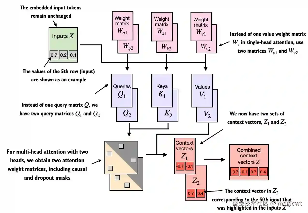
将因果注意力扩展到多头注意力。首先,可以直观地通过堆叠多个CausalAttention模块来构建多头注意力模块。如图18所示,其中包含两个"头"。多头注意力模块包含两个堆叠在一起的单头注意力模块。因此,我们不是使用一个单一的矩阵 Wv来计算值矩阵,而是在一个有两个头的多头注意模块中,现在有两个值权重矩阵: Wv1 和 Wv2。这同样适用于其他的权重矩阵,比如 Wq 和 Wk。我们得到了两组上下文向量 Z1 和 Z2,最终可以将它们合并成一个单一的上下文向量矩阵 Z。
多头注意力的主要思想是多次(并行)运行注意力机制,每次使用学到的不同的线性投影------这些投影是通过将输入数据(比如注意力机制中的查询向量、键向量和值向量)乘以权重矩阵得到的。
多头注意力的一个简单的实现方式是初始化多个前面已实现的因果注意力层,将词元向量序列同时输入到多个因果注意力层中,得到多个上下文向量序列,再将多个上下文向量序列拼接在一起,得到最终的上下文向量序列。
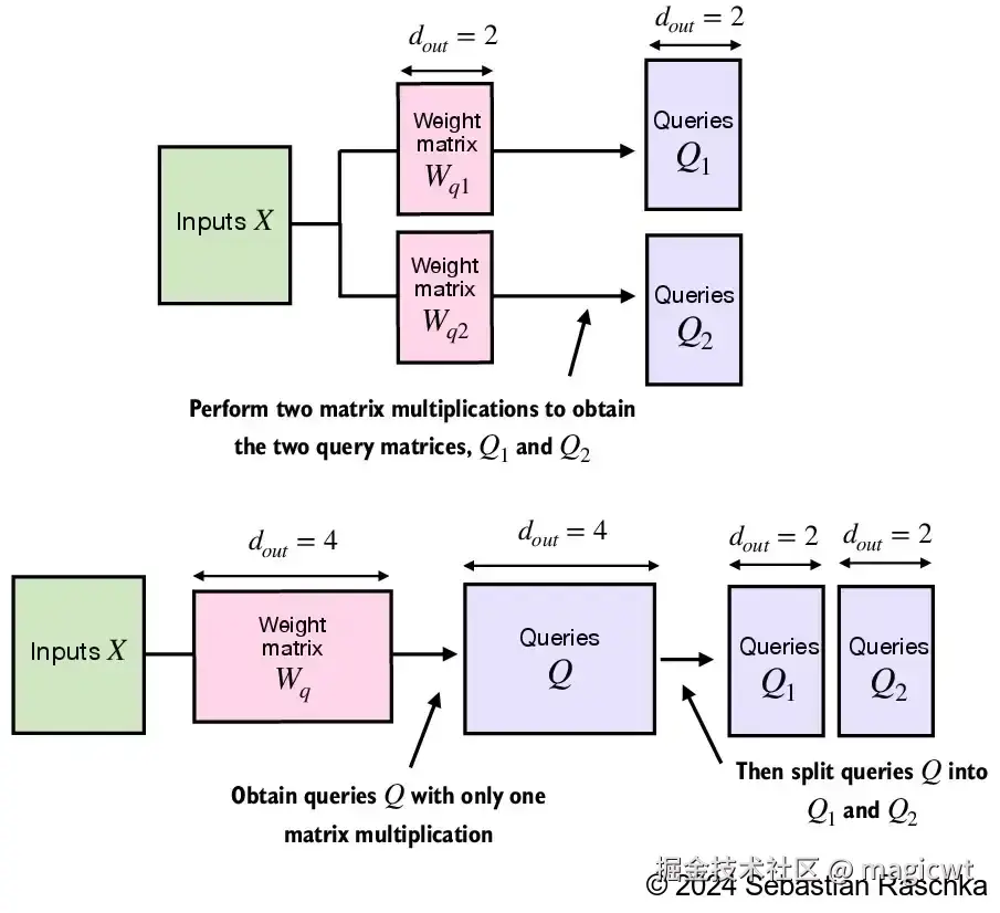
另外一种多头注意力的实现,MultiHeadAttention类会将多头功能整合到一个类内。它通过重新调整投影后的查询张量、键张量和值张量的形状,将输入分为多个头,然后在计算注意力后合并这些头的结果。
多头注意力的两种实现的示意如图19所示。
多头注意力的第二种实现的代码如下所示:
python
import torch
import torch.nn as nn

# 多头注意力实现
class MultiHeadAttention(nn.Module):
    def __init__(self, d_in, d_out, context_length, dropout, num_heads, qkv_bias=False):
        super().__init__()
        assert (d_out % num_heads == 0), \
            "d_out must be divisible by num_heads"

        self.d_out = d_out
        self.num_heads = num_heads
        self.head_dim = d_out // num_heads # Reduce the projection dim to match desired output dim

        self.W_query = nn.Linear(d_in, d_out, bias=qkv_bias)
        self.W_key = nn.Linear(d_in, d_out, bias=qkv_bias)
        self.W_value = nn.Linear(d_in, d_out, bias=qkv_bias)
        self.out_proj = nn.Linear(d_out, d_out)  # Linear layer to combine head outputs
        self.dropout = nn.Dropout(dropout)
        self.register_buffer(
            "mask",
            torch.triu(torch.ones(context_length, context_length),
                       diagonal=1)
        )

    def forward(self, x):
        b, num_tokens, d_in = x.shape
        # As in `CausalAttention`, for inputs where `num_tokens` exceeds `context_length`,
        # this will result in errors in the mask creation further below.
        # In practice, this is not a problem since the LLM (chapters 4-7) ensures that inputs
        # do not exceed `context_length` before reaching this forwar

        keys = self.W_key(x) # Shape: (b, num_tokens, d_out)
        queries = self.W_query(x)
        values = self.W_value(x)

        # We implicitly split the matrix by adding a `num_heads` dimension
        # Unroll last dim: (b, num_tokens, d_out) -> (b, num_tokens, num_heads, head_dim)
        # 对键向量进行拆分,原键向量张量的维度是(批次数,词元序列长度,键向量维度),拆分后的键向量张量的维度是(批次数,词元序列长度,头数,每个头中的键向量维度)
        keys = keys.view(b, num_tokens, self.num_heads, self.head_dim)
        # 对值向量进行拆分,原值向量张量的维度是(批次数,词元序列长度,值向量维度),拆分后的值向量张量的维度是(批次数,词元序列长度,头数,每个头中的值向量维度)
        values = values.view(b, num_tokens, self.num_heads, self.head_dim)
        # 对查询向量进行拆分,原查询向量张量的维度是(批次数,词元序列长度,查询向量维度),拆分后的查询向量张量的维度是(批次数,词元序列长度,头数,每个头中的查询向量维度)
        queries = queries.view(b, num_tokens, self.num_heads, self.head_dim)

        # Transpose: (b, num_tokens, num_heads, head_dim) -> (b, num_heads, num_tokens, head_dim)
        # 交换键向量张量的维度,由(批次数,词元序列长度,头数,每个头中的键向量维度)调整为(批次数,头数,词元序列长度,每个头中的键向量维度)
        keys = keys.transpose(1, 2)
        # 交换查询向量张量的维度,由(批次数,词元序列长度,头数,每个头中的查询向量维度)调整为(批次数,头数,词元序列长度,每个头中的查询向量维度)
        queries = queries.transpose(1, 2)
        # 交换值向量张量的维度,由(批次数,词元序列长度,头数,每个头中的值向量维度)调整为(批次数,头数,词元序列长度,每个头中的值向量维度)
        values = values.transpose(1, 2)

        # 通过查询向量和键向量的点积计算注意力得分,注意力得分的张量维度是(批次数,头数,词元序列长度,词元序列长度)
        # Compute scaled dot-product attention (aka self-attention) with a causal mask
        attn_scores = queries @ keys.transpose(2, 3)  # Dot product for each head

        # Original mask truncated to the number of tokens and converted to boolean
        mask_bool = self.mask.bool()[:num_tokens, :num_tokens]

        # Use the mask to fill attention scores
        attn_scores.masked_fill_(mask_bool, -torch.inf)

        # 计算注意力权重,计算逻辑和因果注意力实现中的逻辑一致,并进行dropout,注意力权重的张量维度是(批次数,头数,词元序列长度,词元序列长度)
        attn_weights = torch.softmax(attn_scores / keys.shape[-1]**0.5, dim=-1)
        attn_weights = self.dropout(attn_weights)
        print("多头注意力权重:\n", attn_weights)

        # 根据注意力权重和值向量计算上下文向量,计算逻辑和因果注意力实现中的逻辑一致,上下文向量的张量维度是(批次数,头数,词元序列长度,每个头中的上下文向量维度)
        # 并交换上下文向量张量的维度,由(批次数,头数,词元序列长度,每个头中的上下文向量维度)调整为(批次数,词元序列长度,头数,每个头中的上下文向量维度)
        # Shape: (b, num_tokens, num_heads, head_dim)
        context_vec = (attn_weights @ values).transpose(1, 2)
        print("合并前的上下文向量:\n", context_vec)

        # 拼接各个头中的上下文向量,得到最终由多头注意力输出的上下文向量,最终上下文向量张量的维度是(批次数,词元序列长度,上下文向量维度)
        # Combine heads, where self.d_out = self.num_heads * self.head_dim
        context_vec = context_vec.contiguous().view(b, num_tokens, self.d_out)
        print("合并后的上下文向量:\n", context_vec)
        context_vec = self.out_proj(context_vec) # optional projection

        return context_vec

torch.manual_seed(123)
# 模拟文本"Your journey starts with one step"的词元向量序列
inputs = torch.tensor(
  [[0.43, 0.15, 0.89], # Your     (x^1)
   [0.55, 0.87, 0.66], # journey  (x^2)
   [0.57, 0.85, 0.64], # starts   (x^3)
   [0.22, 0.58, 0.33], # with     (x^4)
   [0.77, 0.25, 0.10], # one      (x^5)
   [0.05, 0.80, 0.55]] # step     (x^6)
)
# 使用两个输入构成批次
batch = torch.stack((inputs, inputs), dim=0)
# 词元向量序列长度为6
context_length = batch.shape[1]
# 词元向量维度为3
d_in = inputs.shape[1] # the input embedding size, d=3
# 上下文向量维度为2
d_out = 2 # the output embedding size, d=2
# 输出经过多头注意力层后的上下文向量,有两个上下文向量序列,每个上下文向量序列的长度和输入的词元向量序列长度一致,为6
mha = MultiHeadAttention(d_in, d_out, context_length, 0.0, num_heads=2)
context_vecs = mha(batch)
print(context_vecs)
print("context_vecs.shape:", context_vecs.shape)
代码执行结果如下所示:
plain
多头注意力权重:
 tensor([[[[1.0000, 0.0000, 0.0000, 0.0000, 0.0000, 0.0000],
          [0.4776, 0.5224, 0.0000, 0.0000, 0.0000, 0.0000],
          [0.3140, 0.3434, 0.3426, 0.0000, 0.0000, 0.0000],
          [0.2458, 0.2559, 0.2556, 0.2427, 0.0000, 0.0000],
          [0.1967, 0.2090, 0.2087, 0.1929, 0.1927, 0.0000],
          [0.1649, 0.1726, 0.1724, 0.1625, 0.1624, 0.1653]],

         [[1.0000, 0.0000, 0.0000, 0.0000, 0.0000, 0.0000],
          [0.4988, 0.5012, 0.0000, 0.0000, 0.0000, 0.0000],
          [0.3325, 0.3338, 0.3337, 0.0000, 0.0000, 0.0000],
          [0.2463, 0.2505, 0.2504, 0.2528, 0.0000, 0.0000],
          [0.2025, 0.1995, 0.1996, 0.1978, 0.2007, 0.0000],
          [0.1625, 0.1667, 0.1666, 0.1691, 0.1650, 0.1702]]],


        [[[1.0000, 0.0000, 0.0000, 0.0000, 0.0000, 0.0000],
          [0.4776, 0.5224, 0.0000, 0.0000, 0.0000, 0.0000],
          [0.3140, 0.3434, 0.3426, 0.0000, 0.0000, 0.0000],
          [0.2458, 0.2559, 0.2556, 0.2427, 0.0000, 0.0000],
          [0.1967, 0.2090, 0.2087, 0.1929, 0.1927, 0.0000],
          [0.1649, 0.1726, 0.1724, 0.1625, 0.1624, 0.1653]],

         [[1.0000, 0.0000, 0.0000, 0.0000, 0.0000, 0.0000],
          [0.4988, 0.5012, 0.0000, 0.0000, 0.0000, 0.0000],
          [0.3325, 0.3338, 0.3337, 0.0000, 0.0000, 0.0000],
          [0.2463, 0.2505, 0.2504, 0.2528, 0.0000, 0.0000],
          [0.2025, 0.1995, 0.1996, 0.1978, 0.2007, 0.0000],
          [0.1625, 0.1667, 0.1666, 0.1691, 0.1650, 0.1702]]]],
       grad_fn=<SoftmaxBackward0>)
合并前的上下文向量:
 tensor([[[[-0.4519],
          [ 0.2216]],

         [[-0.5889],
          [ 0.0122]],

         [[-0.6313],
          [-0.0576]],

         [[-0.5685],
          [-0.0832]],

         [[-0.5541],
          [-0.0964]],

         [[-0.5311],
          [-0.1077]]],


        [[[-0.4519],
          [ 0.2216]],

         [[-0.5889],
          [ 0.0122]],

         [[-0.6313],
          [-0.0576]],

         [[-0.5685],
          [-0.0832]],

         [[-0.5541],
          [-0.0964]],

         [[-0.5311],
          [-0.1077]]]], grad_fn=<TransposeBackward0>)
合并后的上下文向量:
 tensor([[[-0.4519,  0.2216],
         [-0.5889,  0.0122],
         [-0.6313, -0.0576],
         [-0.5685, -0.0832],
         [-0.5541, -0.0964],
         [-0.5311, -0.1077]],

        [[-0.4519,  0.2216],
         [-0.5889,  0.0122],
         [-0.6313, -0.0576],
         [-0.5685, -0.0832],
         [-0.5541, -0.0964],
         [-0.5311, -0.1077]]], grad_fn=<ViewBackward0>)
tensor([[[0.3190, 0.4858],
         [0.2943, 0.3897],
         [0.2856, 0.3593],
         [0.2693, 0.3873],
         [0.2639, 0.3928],
         [0.2575, 0.4028]],

        [[0.3190, 0.4858],
         [0.2943, 0.3897],
         [0.2856, 0.3593],
         [0.2693, 0.3873],
         [0.2639, 0.3928],
         [0.2575, 0.4028]]], grad_fn=<ViewBackward0>)
context_vecs.shape: torch.Size([2, 6, 2])
从头实现GPT模型进行文本生成
使用层归一化进行归一化激活
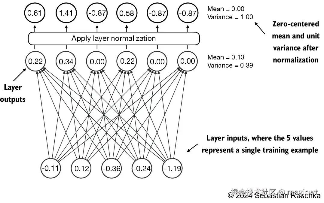
通过使用层归一化,提高神经网络训练的稳定性和效率。层归一化的主要思想是调整神经网络层的激活(输出),使其均值为 0 且方差(单位方差)为 1。这种调整有助于加速权重的有效收敛,并确保训练过程的一致性和可靠性。
层归一化的代码如下所示:
python
import torch
import torch.nn as nn

class LayerNorm(nn.Module):
    def __init__(self, emb_dim):
        super().__init__()
        self.eps = 1e-5
        self.scale = nn.Parameter(torch.ones(emb_dim))
        self.shift = nn.Parameter(torch.zeros(emb_dim))

    def forward(self, x):
        mean = x.mean(dim=-1, keepdim=True)
        var = x.var(dim=-1, keepdim=True, unbiased=False)
        norm_x = (x - mean) / torch.sqrt(var + self.eps)
return self.scale * norm_x + self.shift层归一化的具体实现作用在输入张量x的最后一个维度上,该维度对应于嵌入维度(emb_dim)。变量eps是一个小常数,在归一化过程中会被加到方差上以防止除零错误。scale和shift是两个可训练的参数(与输入维度相同),如果在训练过程中发现调整它们可以改善模型的训练任务表现,那么大语言模型会自动进行调整。这使得模型能够学习适合其数据处理的最佳缩放和偏移。
实现具有GELU激活函数的前馈神经网络
GELU和SwiGLU是更为复杂且平滑的激活函数,分别结合了高斯分布和Sigmoid门控线性单元。与较为简单的 ReLU激活函数相比,它们能够提升深度学习模型的性能。GELU激活函数可以通过多种方式实现,其精确的定义为:
GELU(x)=x⋅Φ(x)
其中, Φ(x)是标准高斯分布的累积分布函数。然而,在实际操作中,通常我们会使用一种计算量较小的近似实现(原始的 GPT-2 模型也是使用这种通过曲线拟合得到的近似方法进行训练的):
GELU(x)≈0.5⋅x⋅(1+tanhπ2 ⋅(x+0.044715⋅x3))
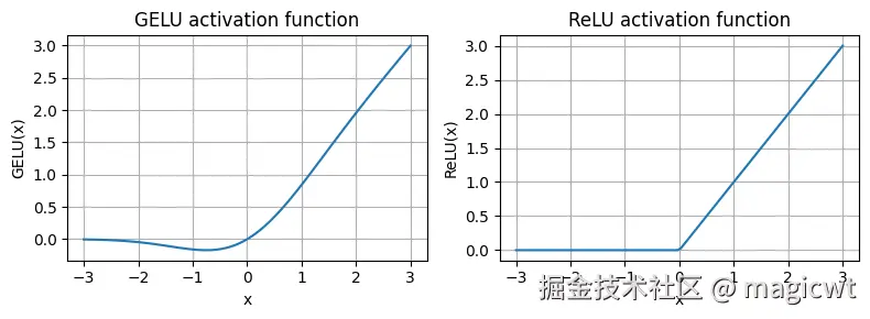
GELU和ReLU的函数曲线如图21所示,ReLU是一个分段线性函数,当输入为正数时直接输出输入值,否则输出 0。GELU则是一个平滑的非线性函数,它近似ReLU,但在几乎所有负值上都有非零梯度。
GELU的平滑特性可以在训练过程中带来更好的优化效果,因为它允许模型参数进行更细微的调整。相比之下,ReLU在零点处有一个尖锐的拐角,有时会使得优化过程更加困难,特别是在深度或复杂的网络结构中。此外,ReLU对负输入的输出为0,而GELU对负输入会输出一个小的非零值。这意味着在训练过程中,接收到负输入的神经元仍然可以参与学习,只是贡献程度不如正输入大。
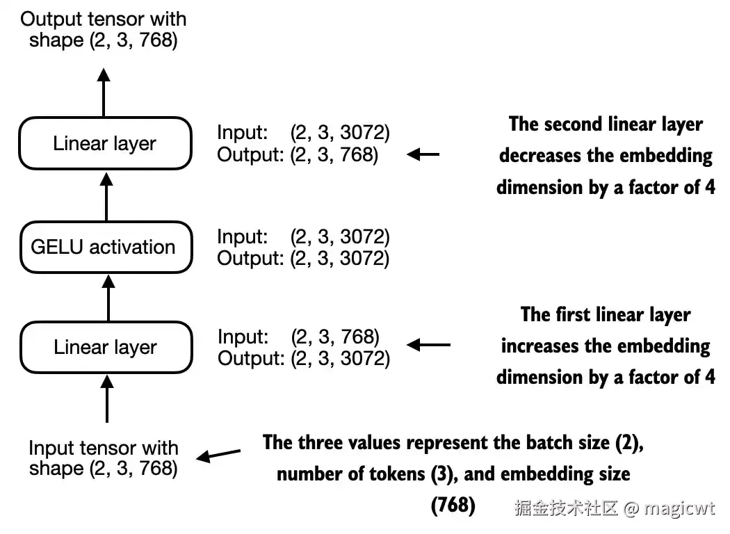
FeedForward模块是一个小型神经网络,由两个线性层和一个GELU激活函数组成,如图22所示。
第一个线性层的输入张量的维度是(批次数,词元序列长度,词元嵌入维度)(2,3,768),输出张量的维度(批次数,词元序列长度,词元嵌入维度)(2,3,3072),输入时词元嵌入维度是768,输出时词元嵌入维度是3072,增加至输入的4倍。
激活函数的输入张量的维度是(批次数,词元序列长度,词元嵌入维度)(2,3,3072),输出张量的维度是(批次数,词元序列长度,词元嵌入维度)(2,3,3072),输入和输出的维度无变化,但通过激活函数引入了非线性。
第二个线性层的输入张量的维度是(批次数,词元序列长度,词元嵌入维度)(2,3,3072),输出张量的维度(批次数,词元序列长度,词元嵌入维度)(2,3,768),输入时词元嵌入维度是3072,输出时词元嵌入维度是768,减少至输入的1/4。
整体看FeedForward模块,输入和输出张量的维度保持不变,但通过激活函数引入了非线性。FeedForward模块在提升模型学习和泛化能力方面非常关键。虽然该模块的输入和输出维度保持一致,但它通过第一个线性层将嵌入维度扩展到了更高的维度,如图22所示。扩展之后,应用非线性GELU激活函数,然后通过第二个线性变换将维度缩回原始大小。这种设计允许模型探索更丰富的表示空间。
FeedForward模块的代码如下所示:
python
import torch
import torch.nn as nn

class FeedForward(nn.Module):
    def __init__(self, cfg):
        super().__init__()
        self.layers = nn.Sequential(
            nn.Linear(cfg["emb_dim"], 4 * cfg["emb_dim"]),
            GELU(),
            nn.Linear(4 * cfg["emb_dim"], cfg["emb_dim"]),
        )

    def forward(self, x):
        return self.layers(x)
增加残差连接
这是通过将某一层的输入直接叠加到该层的输出中实现的,其能够解决网络层数过多时的梯度消失问题。
连接Transformer块中的注意力层和线性层
首先,安装llms_from_scratch,里面包含了书中实现的一些类和方法:
shell
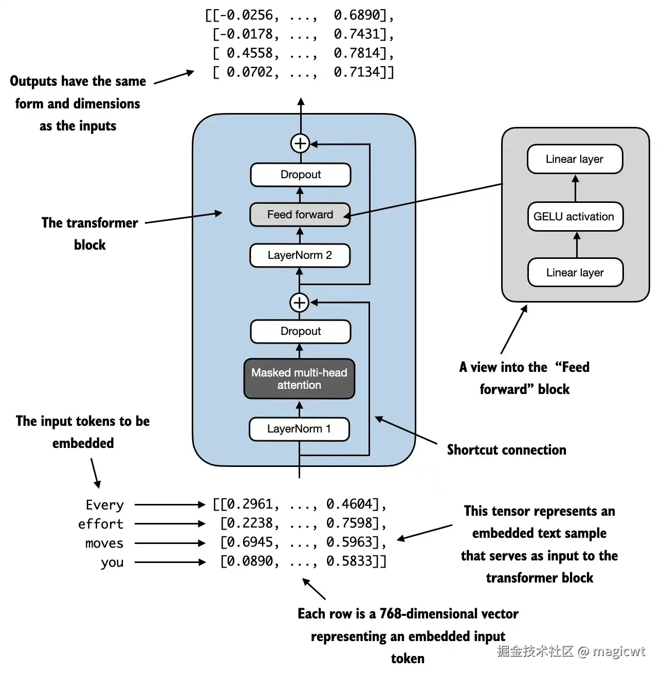
uv pip install llms_from_scratch实现Transformer块,这是GPT和其他大语言模型架构的基本构建块。在参数量为1.24亿的GPT-2架构中,这个块被重复多次,它结合了之前提及的多个概念:多头注意力、层归一化、dropout、前馈层和GELU激活函数。
Transformer块的结构如图23所示。Transformer块的核心思想是,自注意力机制在多头注意力块中用于识别和分析输入序列中元素之间的关系。相比之下,前馈神经网络则在每个位置上对数据进行单独的修改。这种组合不仅提供了对输入更细致的理解和处理,而且提升了模型处理复杂数据模式的整体能力。
Transformer块的代码如下所示:
python
import torch
import torch.nn as nn
from llms_from_scratch.ch03 import MultiHeadAttention

class TransformerBlock(nn.Module):
    def __init__(self, cfg):
        super().__init__()
        # 使用MultiHeadAttention定义Transformer块中的多头注意力层
        self.att = MultiHeadAttention(
            d_in=cfg["emb_dim"],
            d_out=cfg["emb_dim"],
            context_length=cfg["context_length"],
            num_heads=cfg["n_heads"],
            dropout=cfg["drop_rate"],
            qkv_bias=cfg["qkv_bias"])
        # 使用FeedForward定义Transformer块中的前馈全连接网络层
        self.ff = FeedForward(cfg)
        # 使用LayerNorm定义Transformer块中的层归一化层
        self.norm1 = LayerNorm(cfg["emb_dim"])
        self.norm2 = LayerNorm(cfg["emb_dim"])
        self.drop_shortcut = nn.Dropout(cfg["drop_rate"])

    def forward(self, x):
        # Shortcut connection for attention block
        shortcut = x
        # 对Transformer块的输入进行层归一化
        x = self.norm1(x)
        # 将层归一化层的输出输入多头注意力层
        x = self.att(x)  # Shape [batch_size, num_tokens, emb_size]
        # 对多头注意力层的输出进行dropout
        x = self.drop_shortcut(x)
        # 将多头注意力层的输出(经过dropout后)与层归一化前的输入进行相加,实现残差连接
        x = x + shortcut  # Add the original input back

        # Shortcut connection for feed forward block
        shortcut = x
        # 将上一环节的输出进行层归一化
        x = self.norm2(x)
        # 将层归一化的输出输入前馈全连接网络层
        x = self.ff(x)
        # 对前馈全连接网络层的输出进行dropout
        x = self.drop_shortcut(x)
        # 将前馈全连接网络层的输出(经过dropout后)与层归一化前的输入进行相加,实现残差连接
        x = x + shortcut  # Add the original input back

        return x
实现GPT模型
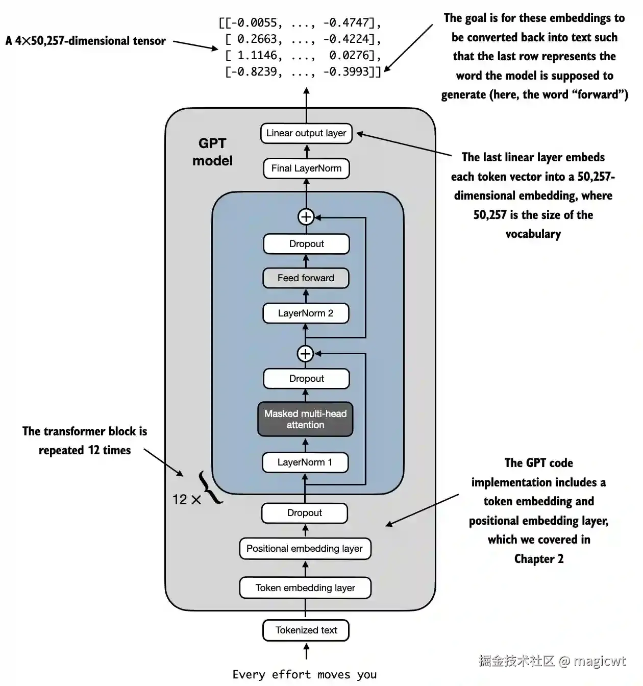
Transformer块在GPT模型架构中被多次重复。在参数量为1.24亿的GPT-2模型中,Transformer块被重复使用12次,这可以通过GPT_CONFIG_124M字典中的n_layers字段进行指定。在最大规模的GPT-2模型(参数量为15.42亿)中,Transformer块被重复使用48次。
在Transformer块之前,增加词元序列的词元和位置的嵌入层,以及dropout层,在Transformer块之后,增加层归一化层和线性输出层,得到GPT模型,如图24所示。
GPT模型的代码如下所示:
python
import torch
import torch.nn as nn

class GPTModel(nn.Module):
    def __init__(self, cfg):
        super().__init__()
        # 定义词元的嵌入层
        self.tok_emb = nn.Embedding(cfg["vocab_size"], cfg["emb_dim"])
        # 定义位置的嵌入层
        self.pos_emb = nn.Embedding(cfg["context_length"], cfg["emb_dim"])
        self.drop_emb = nn.Dropout(cfg["drop_rate"])
        # 定义连续的多个Transformer块
        self.trf_blocks = nn.Sequential(
            *[TransformerBlock(cfg) for _ in range(cfg["n_layers"])])
        # 定义层归一化层
        self.final_norm = LayerNorm(cfg["emb_dim"])
        # 定义线性输出层
        self.out_head = nn.Linear(
            cfg["emb_dim"], cfg["vocab_size"], bias=False
        )

    def forward(self, in_idx):
        batch_size, seq_len = in_idx.shape
        # 将词元通过词元嵌入层转化为词元嵌入向量
        tok_embeds = self.tok_emb(in_idx)
        # 将位置通过位置嵌入层转化为位置嵌入向量
        pos_embeds = self.pos_emb(torch.arange(seq_len, device=in_idx.device))
        # 将词元嵌入向量和位置嵌入向量相加得到最终的词元嵌入向量作为输入
        x = tok_embeds + pos_embeds  # Shape [batch_size, num_tokens, emb_size]
        # 将输入进行dropout
        x = self.drop_emb(x)
        # 将dropout的输出输入Transformer块
        x = self.trf_blocks(x)
        # 将Transformer块的输出进行层归一化
        x = self.final_norm(x)
        # 将层归一化的输出输入线性输出层
        logits = self.out_head(x)
        return logits
生成文本
大语言模型逐步生成文本的过程如图25所示,每次生成一个词元。从初始输入上下文("Hello, I am")开始,模型在每轮迭代中预测下一个词元,并将其添加到输入上下文中以进行下一轮预测。第一轮迭代添加了"a",第二轮迭代添加了"model",第三轮迭代添加了"ready",逐步形成完整的句子。在第6次迭代时,模型生成了完整的句子"Hello, I am a model ready to help."。
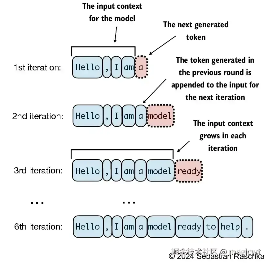
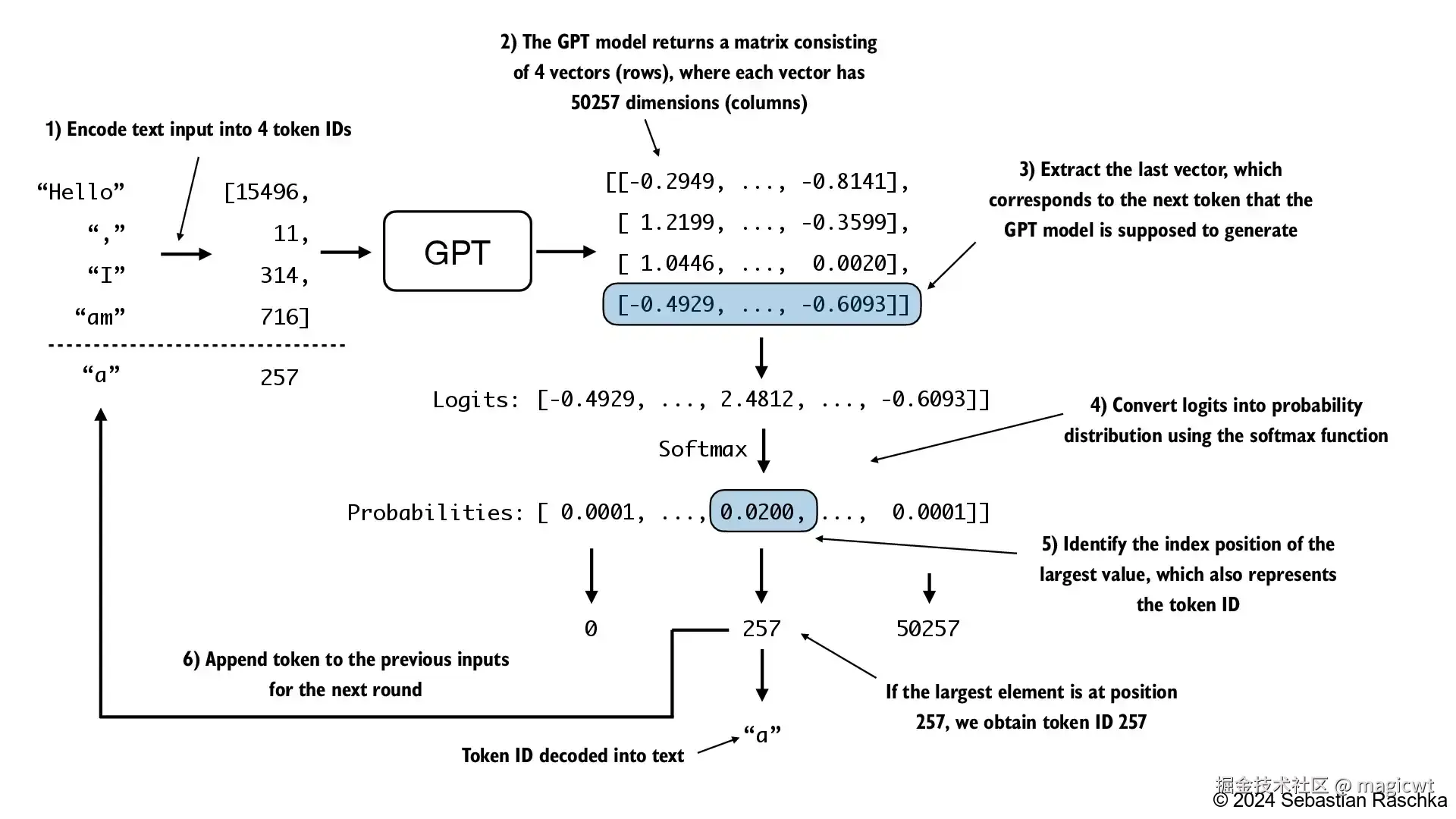
图26说明了GPT模型如何在给定输入的情况下生成下一个词元。在每一步中,模型输出一个矩阵,其中的向量表示有可能的下一个词元。将与下一个词元对应的向量提取出来,该向量的维度与词典的大小一致,并通过Softmax函数将该向量转换为概率分布。在该向量中,找到概率分数最高值的索引,这个索引对应于词元ID。然后将这个词元ID解码为文本,生成序列中的下一个词元。最后,将这个词元附加到之前的输入中,形成新的输入序列,供下一次迭代使用。这个逐步的过程使得模型能够按顺序生成文本,从最初的输入上下文开始构建连贯的短语和句子。实际操作会多次重复这一过程,如图25所示,直至生成预定数量的词元。
文本生成的代码如下所示:
python
def generate_text_simple(model, idx, max_new_tokens, context_size):
    # idx is (batch, n_tokens) array of indices in the current context
    for _ in range(max_new_tokens):

        # Crop current context if it exceeds the supported context size
        # E.g., if LLM supports only 5 tokens, and the context size is 10
        # then only the last 5 tokens are used as context
        idx_cond = idx[:, -context_size:]

        # Get the predictions
        with torch.no_grad():
            logits = model(idx_cond)

        # Focus only on the last time step
        # (batch, n_tokens, vocab_size) becomes (batch, vocab_size)
        logits = logits[:, -1, :]

        # Apply softmax to get probabilities
        probas = torch.softmax(logits, dim=-1)  # (batch, vocab_size)

        # Get the idx of the vocab entry with the highest probability value
        idx_next = torch.argmax(probas, dim=-1, keepdim=True)  # (batch, 1)

        # Append sampled index to the running sequence
        idx = torch.cat((idx, idx_next), dim=1)  # (batch, n_tokens+1)

    return idx
在无标签数据上进行预训练
评估文本生成模型
对于上一节定义的GPT模型,如果不进行训练,直接基于一段文本"Every effort moves you",由GPT模型预测后续的文本,代码如下所示:
python
import tiktoken
import torch

from llms_from_scratch.ch04 import generate_text_simple
from llms_from_scratch.ch04 import GPTModel

GPT_CONFIG_124M = {
    "vocab_size": 50257,   # Vocabulary size
    "context_length": 256, # Shortened context length (orig: 1024)
    "emb_dim": 768,        # Embedding dimension
    "n_heads": 12,         # Number of attention heads
    "n_layers": 12,        # Number of layers
    "drop_rate": 0.1,      # Dropout rate
    "qkv_bias": False      # Query-key-value bias
}

torch.manual_seed(123)
model = GPTModel(GPT_CONFIG_124M)
model.eval();  # Disable dropout during inference

def text_to_token_ids(text, tokenizer):
    encoded = tokenizer.encode(text, allowed_special={'<|endoftext|>'})
    encoded_tensor = torch.tensor(encoded).unsqueeze(0) # add batch dimension
    return encoded_tensor

def token_ids_to_text(token_ids, tokenizer):
    flat = token_ids.squeeze(0) # remove batch dimension
    return tokenizer.decode(flat.tolist())

start_context = "Every effort moves you"
tokenizer = tiktoken.get_encoding("gpt2")

token_ids = generate_text_simple(
    model=model,
    idx=text_to_token_ids(start_context, tokenizer),
    max_new_tokens=10,
    context_size=GPT_CONFIG_124M["context_length"]
)

print("Output text:\n", token_ids_to_text(token_ids, tokenizer))
由于尚未经过训练,模型还无法生成连贯的文本,执行结果如下所示:
plain
Output text:
 Every effort moves you rentingetic wasnم refres RexMeCHicular stren
为了使得模型能够生成连贯的文本,需要使用训练样本集对模型进行训练,不断调整模型的参数,使得模型在训练样本集和评估样本集的损失函数值逐渐减少。
损失函数一般采用交叉熵损失。
在机器学习和深度学习中,交叉熵损失是一种常用的度量方式,用于衡量两个概率分布之间的差异------通常是标签(在这里是数据集中的词元)的真实分布和模型生成的预测分布(例如,由大语言模型生成的词元概率)之间的差异。
大预言模型的输出是下一个词元是词典中某个词元的概率,其交叉熵损失如下所示:
LCE=−i=1∑nyilogyi^
交叉熵损失中, n表示词典中词元的数量, i表示词典中的第 i个词元, yi表示词典中的第 i个词元是下一个词元的真实概率,若第 i个词元就是真实的下一个词元,则 yi=1,否则 yi=0, y^i表示词典中的第 i个词元是下一个词元的模型预测概率,若第 i个词元就是真实的下一个词元,则 y^i越接近1, LCE越小。
训练大语言模型
将之前已介绍的短篇小说《The Verdict》作为数据集(其中大部分作为训练数据集,小部分作为验证数据集)对GPT模型进行预训练,代码如下所示:
python
# Copyright (c) Sebastian Raschka under Apache License 2.0 (see LICENSE.txt).
# Source for "Build a Large Language Model From Scratch"
# - https://www.manning.com/books/build-a-large-language-model-from-scratch
# Code: https://github.com/rasbt/LLMs-from-scratch
import matplotlib.pyplot as plt
import os
import torch
import urllib.request
import tiktoken
from llms_from_scratch.ch02 import create_dataloader_v1
from llms_from_scratch.ch04 import GPTModel, generate_text_simple
def text_to_token_ids(text, tokenizer):
"""将词元转化词元id"""
encoded = tokenizer.encode(text)
encoded_tensor = torch.tensor(encoded).unsqueeze(0) # add batch dimension
return encoded_tensor
def token_ids_to_text(token_ids, tokenizer):
"""将词元id转化词元"""
flat = token_ids.squeeze(0) # remove batch dimension
return tokenizer.decode(flat.tolist())
def calc_loss_batch(input_batch, target_batch, model, device):
"""计算每个批次模型预估概率和真实概率的交叉熵损失"""
input_batch, target_batch = input_batch.to(device), target_batch.to(device)
logits = model(input_batch)
loss = torch.nn.functional.cross_entropy(logits.flatten(0, 1), target_batch.flatten())
return loss
def calc_loss_loader(data_loader, model, device, num_batches=None):
"""对数据集中的多个批次,计算每个批次模型预估概率和真实概率的交叉熵损失,并计算每个批次交叉熵损失的平均值"""
total_loss = 0.
if len(data_loader) == 0:
return float("nan")
elif num_batches is None:
num_batches = len(data_loader)
else:
num_batches = min(num_batches, len(data_loader))
for i, (input_batch, target_batch) in enumerate(data_loader):
if i < num_batches:
loss = calc_loss_batch(input_batch, target_batch, model, device)
total_loss += loss.item()
else:
break
return total_loss / num_batches
def evaluate_model(model, train_loader, val_loader, device, eval_iter):
"""评估模型,计算模型在训练数据集和测试数据集的交叉熵损失"""
model.eval()
with torch.no_grad():
train_loss = calc_loss_loader(train_loader, model, device, num_batches=eval_iter)
val_loss = calc_loss_loader(val_loader, model, device, num_batches=eval_iter)
model.train()
return train_loss, val_loss
def generate_and_print_sample(model, tokenizer, device, start_context):
"""使用模型进行推理,基于已有文本,预测下一个词元,最多预测50个词元"""
model.eval()
context_size = model.pos_emb.weight.shape[0]
encoded = text_to_token_ids(start_context, tokenizer).to(device)
with torch.no_grad():
token_ids = generate_text_simple(
model=model, idx=encoded,
max_new_tokens=50, context_size=context_size
)
decoded_text = token_ids_to_text(token_ids, tokenizer)
print(decoded_text.replace("\n", " ")) # Compact print format
model.train()
def train_model_simple(model, train_loader, val_loader, optimizer, device, num_epochs,
eval_freq, eval_iter, start_context, tokenizer):
"""对模型进行训练"""
# Initialize lists to track losses and tokens seen
train_losses, val_losses, track_tokens_seen = [], [], []
tokens_seen = 0
global_step = -1
# Main training loop
for epoch in range(num_epochs):
# 对训练数据集重复多次
model.train() # Set model to training mode
for input_batch, target_batch in train_loader:
# 对训练数据集的每个批次
optimizer.zero_grad() # Reset loss gradients from previous batch iteration
# 计算交叉熵损失
loss = calc_loss_batch(input_batch, target_batch, model, device)
# 计算梯度
loss.backward() # Calculate loss gradients
# 反向传播,根据梯度更新模型参数
optimizer.step() # Update model weights using loss gradients
tokens_seen += input_batch.numel()
global_step += 1
# Optional evaluation step
if global_step % eval_freq == 0:
train_loss, val_loss = evaluate_model(
model, train_loader, val_loader, device, eval_iter)
train_losses.append(train_loss)
val_losses.append(val_loss)
track_tokens_seen.append(tokens_seen)
print(f"Ep {epoch+1} (Step {global_step:06d}): "
f"Train loss {train_loss:.3f}, Val loss {val_loss:.3f}")
# 遍历一次训练数据集后,使用模型进行推理
# Print a sample text after each epoch
generate_and_print_sample(
model, tokenizer, device, start_context
)
return train_losses, val_losses, track_tokens_seen
def plot_losses(epochs_seen, tokens_seen, train_losses, val_losses):
"""绘制训练过程中的损失变化曲线"""
fig, ax1 = plt.subplots()
# Plot training and validation loss against epochs
ax1.plot(epochs_seen, train_losses, label="Training loss")
ax1.plot(epochs_seen, val_losses, linestyle="-.", label="Validation loss")
ax1.set_xlabel("Epochs")
ax1.set_ylabel("Loss")
ax1.legend(loc="upper right")
# Create a second x-axis for tokens seen
ax2 = ax1.twiny() # Create a second x-axis that shares the same y-axis
ax2.plot(tokens_seen, train_losses, alpha=0) # Invisible plot for aligning ticks
ax2.set_xlabel("Tokens seen")
fig.tight_layout() # Adjust layout to make room
# plt.show()
def main(gpt_config, settings):
"""定义模型训练主流程"""
torch.manual_seed(123)
device = torch.device("cuda" if torch.cuda.is_available() else "cpu")
##############################
# 下载数据集,即之前已介绍的短篇小说《The Verdict》
# Download data if necessary
##############################
file_path = "the-verdict.txt"
url = "https://raw.githubusercontent.com/rasbt/LLMs-from-scratch/main/ch02/01_main-chapter-code/the-verdict.txt"
if not os.path.exists(file_path):
with urllib.request.urlopen(url) as response:
text_data = response.read().decode('utf-8')
with open(file_path, "w", encoding="utf-8") as file:
file.write(text_data)
else:
with open(file_path, "r", encoding="utf-8") as file:
text_data = file.read()
##############################
# 初始化模型,即之前已定义的GPTModel
# Initialize model
##############################
model = GPTModel(gpt_config)
model.to(device) # no assignment model = model.to(device) necessary for nn.Module classes
optimizer = torch.optim.AdamW(
model.parameters(), lr=settings["learning_rate"], weight_decay=settings["weight_decay"]
)
##############################
# 将数据集划分为训练数据集和评估数据集
# Set up dataloaders
##############################
# Train/validation ratio
train_ratio = 0.90
split_idx = int(train_ratio * len(text_data))
train_loader = create_dataloader_v1(
text_data[:split_idx],
batch_size=settings["batch_size"],
max_length=gpt_config["context_length"],
stride=gpt_config["context_length"],
drop_last=True,
shuffle=True,
num_workers=0
)
val_loader = create_dataloader_v1(
text_data[split_idx:],
batch_size=settings["batch_size"],
max_length=gpt_config["context_length"],
stride=gpt_config["context_length"],
drop_last=False,
shuffle=False,
num_workers=0
)
##############################
# 训练模型
# Train model
##############################
tokenizer = tiktoken.get_encoding("gpt2")
train_losses, val_losses, tokens_seen = train_model_simple(
model, train_loader, val_loader, optimizer, device,
num_epochs=settings["num_epochs"], eval_freq=5, eval_iter=5,
start_context="Every effort moves you", tokenizer=tokenizer
)
return train_losses, val_losses, tokens_seen, model
if __name__ == "__main__":
# 模型和训练的超参数
#
# 模型的超参数
# 词典大小:50257
# 上下文长度:256
# 嵌入向量维度:768
# 头数:12
# 层数:12
#
# 训练的超参数
# 学习率:0.0005
# 数据集重复次数:10
# 批次大小:2
GPT_CONFIG_124M = {
"vocab_size": 50257, # Vocabulary size
"context_length": 256, # Shortened context length (orig: 1024)
"emb_dim": 768, # Embedding dimension
"n_heads": 12, # Number of attention heads
"n_layers": 12, # Number of layers
"drop_rate": 0.1, # Dropout rate
"qkv_bias": False # Query-key-value bias
}
OTHER_SETTINGS = {
"learning_rate": 0.0004,
"num_epochs": 10,
"batch_size": 2,
"weight_decay": 0.1
}
###########################
# 执行模型训练主流程
# Initiate training
###########################
train_losses, val_losses, tokens_seen, model = main(GPT_CONFIG_124M, OTHER_SETTINGS)
###########################
# After training
###########################
# 绘制训练过程中的损失变化曲线
# Plot results
epochs_tensor = torch.linspace(0, OTHER_SETTINGS["num_epochs"], len(train_losses))
plot_losses(epochs_tensor, tokens_seen, train_losses, val_losses)
plt.savefig("loss.pdf")
# 保存并加载模型
# Save and load model
torch.save(model.state_dict(), "model.pth")
model = GPTModel(GPT_CONFIG_124M)
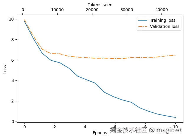
model.load_state_dict(torch.load("model.pth", weights_only=True))训练过程中的损失变化曲线如图27所示,训练集损失和验证集损失整体趋势是逐渐减小。在训练开始阶段,训练集损失和验证集损失急剧下降,这表明模型正在学习。然而,在第二轮之后,训练集损失继续下降,验证集损失则停滞不前。这表明模型仍在学习,但在第二轮之后开始对训练集过拟合。这种记忆现象其实是可以预料到的,因为我们使用了一个非常小的训练数据集,并且对模型进行了多轮训练。通常,在更大的数据集上训练模型时,只训练一轮是很常见的做法。
训练过程中,每遍历一次训练数据集后,使用模型进行推理,输出的结果如下所示:
plain
Ep 1 (Step 000000): Train loss 9.781, Val loss 9.933
Ep 1 (Step 000005): Train loss 8.111, Val loss 8.339
Every effort moves you,,,,,,,,,,,,.
Ep 2 (Step 000010): Train loss 6.661, Val loss 7.048
Ep 2 (Step 000015): Train loss 5.961, Val loss 6.616
Every effort moves you, and, and, and, and, and, and, and, and, and, and, and, and, and, and, and, and, and, and, and, and, and, and,, and, and,
Ep 3 (Step 000020): Train loss 5.726, Val loss 6.600
Ep 3 (Step 000025): Train loss 5.201, Val loss 6.348
Every effort moves you, and I had been.
Ep 4 (Step 000030): Train loss 4.417, Val loss 6.278
Ep 4 (Step 000035): Train loss 4.069, Val loss 6.226
Every effort moves you know the                          "I he had the donkey and I had the and I had the donkey and down the room, I had
Ep 5 (Step 000040): Train loss 3.732, Val loss 6.160
Every effort moves you know it was not that the picture--I had the fact by the last I had been--his, and in the            "Oh, and he said, and down the room, and in
Ep 6 (Step 000045): Train loss 2.850, Val loss 6.179
Ep 6 (Step 000050): Train loss 2.427, Val loss 6.141
Every effort moves you know," was one of the picture. The--I had a little of a little: "Yes, and in fact, and in the picture was, and I had been at my elbow and as his pictures, and down the room, I had
Ep 7 (Step 000055): Train loss 2.104, Val loss 6.134
Ep 7 (Step 000060): Train loss 1.882, Val loss 6.233
Every effort moves you know," was one of the picture for nothing--I told Mrs.  "I was no--as! The women had been, in the moment--as Jack himself, as once one had been the donkey, and were, and in his
Ep 8 (Step 000065): Train loss 1.320, Val loss 6.238
Ep 8 (Step 000070): Train loss 0.985, Val loss 6.242
Every effort moves you know," was one of the axioms he had been the tips of a self-confident moustache, I felt to see a smile behind his close grayish beard--as if he had the donkey. "strongest," as his
Ep 9 (Step 000075): Train loss 0.717, Val loss 6.293
Ep 9 (Step 000080): Train loss 0.541, Val loss 6.393
Every effort moves you?"  "Yes--quite insensible to the irony. She wanted him vindicated--and by me!"  He laughed again, and threw back the window-curtains, I had the donkey. "There were days when I
Ep 10 (Step 000085): Train loss 0.391, Val loss 6.452
Every effort moves you know," was one of the axioms he laid down across the Sevres and silver of an exquisitely appointed luncheon-table, when, on a later day, I had again run over from Monte Carlo; and Mrs. Gis
在开始阶段,模型只能在起始上下文后添加逗号(Every effort moves you,,,,,,,,,,,,)或重复单词and。在训练结束时,它已经可以生成语法正确的文本。
控制随机性的解码策略
大语言模型的输出是下一个词元是词典中某个词元的概率,经过预训练后,模型已经比较能够准确预测下一个词元,即模型对于正确词元的概率预测值一般最大,将同一个文本多次输入模型,则模型每次均选择概率预测值最大的词元,从而输出相同的文本,但实际我们在使用各类大语言模型时,一般将同一个文本多次输入模型,会得到不同的输出。大语言模型如何在保证一定准确性的同时,实现多样化的输出呢"
在之前的generate_text_simple函数中,我们总是使用torch.argmax(也称为贪婪解码)来采样具有最高概率的词元作为下一个词元,代码如下所示:
python
torch.argmax(probas, dim=-1, keepdim=True)为了生成更多样化的文本,可以用一个从概率分布(这里是大语言模型在预测下一个词元时为词典中每个词元生成的概率分数)中采样的函数来取代argmax。具体可以使用PyTorch中的multinomial函数替换argmax来实现这个概率采样过程,代码如下所示:
python
next_token_id = torch.multinomial(probas, num_samples=1).item()通过一个被称为温度缩放的概念,可以进一步控制分布和选择过程。温度缩放指的是将logits除以一个大于0的数,即temperature,然后在对缩放后的logits(即scaled_logits)通过Softmax函数得到词典中各个词元的概率,代码如下所示:
python
def softmax_with_temperature(logits, temperature):
    scaled_logits = logits / temperature
    return torch.softmax(scaled_logits, dim=0)
温度大于1会导致词元概率更加均匀分布,温度小于1则会导致更加自信(更尖锐或更陡峭)的分布。
应用比较小的温度(例如0.1)会导致更集中的分布,使得multinomial函数几乎100%选择最可能的词元(这里是forward),接近于argmax函数的行为。相反地,应用比较大的温度(例如5)会导致更均匀的分布,使得其他词元更容易被选中。这可以为生成的文本增加更多变化,但也更容易生成无意义的文本。
使用更偏随机性的解码策略生成文本的代码如下所示:
python
import torch
import tiktoken

from llms_from_scratch.ch04 import GPTModel, generate_text_simple

def text_to_token_ids(text, tokenizer):
    """将词元转化词元id"""
    encoded = tokenizer.encode(text)
    encoded_tensor = torch.tensor(encoded).unsqueeze(0)  # add batch dimension
    return encoded_tensor

def token_ids_to_text(token_ids, tokenizer):
    """将词元id转化词元"""
    flat = token_ids.squeeze(0)  # remove batch dimension
    return tokenizer.decode(flat.tolist())

def generate(model, idx, max_new_tokens, context_size, temperature=0.0, top_k=None, eos_id=None):

    # For-loop is the same as before: Get logits, and only focus on last time step
    for _ in range(max_new_tokens):
        idx_cond = idx[:, -context_size:]
        with torch.no_grad():
            logits = model(idx_cond)
        logits = logits[:, -1, :]

        # New: Filter logits with top_k sampling
        if top_k is not None:
            # Keep only top_k values
            top_logits, _ = torch.topk(logits, top_k)
            min_val = top_logits[:, -1]
            logits = torch.where(logits < min_val, torch.tensor(float("-inf")).to(logits.device), logits)

        # New: Apply temperature scaling
        if temperature > 0.0:
            logits = logits / temperature

            # Apply softmax to get probabilities
            probs = torch.softmax(logits, dim=-1)  # (batch_size, context_len)

            # Sample from the distribution
            idx_next = torch.multinomial(probs, num_samples=1)  # (batch_size, 1)

        # Otherwise same as before: get idx of the vocab entry with the highest logits value
        else:
            idx_next = torch.argmax(logits, dim=-1, keepdim=True)  # (batch_size, 1)

        if idx_next == eos_id:  # Stop generating early if end-of-sequence token is encountered and eos_id is specified
            break

        # Same as before: append sampled index to the running sequence
        idx = torch.cat((idx, idx_next), dim=1)  # (batch_size, num_tokens+1)

    return idx


if __name__ == "__main__":

    # 模型和训练的超参数
    #
    # 模型的超参数
    # 词典大小:50257
    # 上下文长度:256
    # 嵌入向量维度:768
    # 头数:12
    # 层数:12
    GPT_CONFIG_124M = {
        "vocab_size": 50257,    # Vocabulary size
        "context_length": 256,  # Shortened context length (orig: 1024)
        "emb_dim": 768,         # Embedding dimension
        "n_heads": 12,          # Number of attention heads
        "n_layers": 12,         # Number of layers
        "drop_rate": 0.1,       # Dropout rate
        "qkv_bias": False       # Query-key-value bias
    }

    model = GPTModel(GPT_CONFIG_124M)
    model.load_state_dict(torch.load("model.pth", weights_only=True))
    model.to("cpu")
    model.eval()

    tokenizer = tiktoken.get_encoding("gpt2")

    torch.manual_seed(123)

    token_ids = generate(
        model=model,
        idx=text_to_token_ids("Every effort moves you", tokenizer),
        max_new_tokens=15,
        context_size=GPT_CONFIG_124M["context_length"],
        temperature=1.4,
        top_k=25
    )

    print("Output text:\n", token_ids_to_text(token_ids, tokenizer))
代码执行结果如下所示:
python
Every effort moves you stand to work on surprise, a one of us had gone with random-《从零构建大模型》通过上述的介绍,手把手带领读者在个人消费级的电脑上实现了一个简单的大语言模型的预训练。后续的介绍,还包括如何加载OpenAI公开的GPT-2的模型参数,并在此基础上进行模型微调。
大语言模型经过这几年的飞速发展,已在上述介绍的基本模型结构的基础上,进一步在强化学习微调、混合专家网络、训练框架加速等多个方面不断深入,不断取得效果和性能的突破。但通过《从零构建大模型》的介绍,读者可以了解大语言模型的基本原理,对大语言模型有一个初步但全面的了解。