基于线性判别LDA实现鸢尾花分类器
-
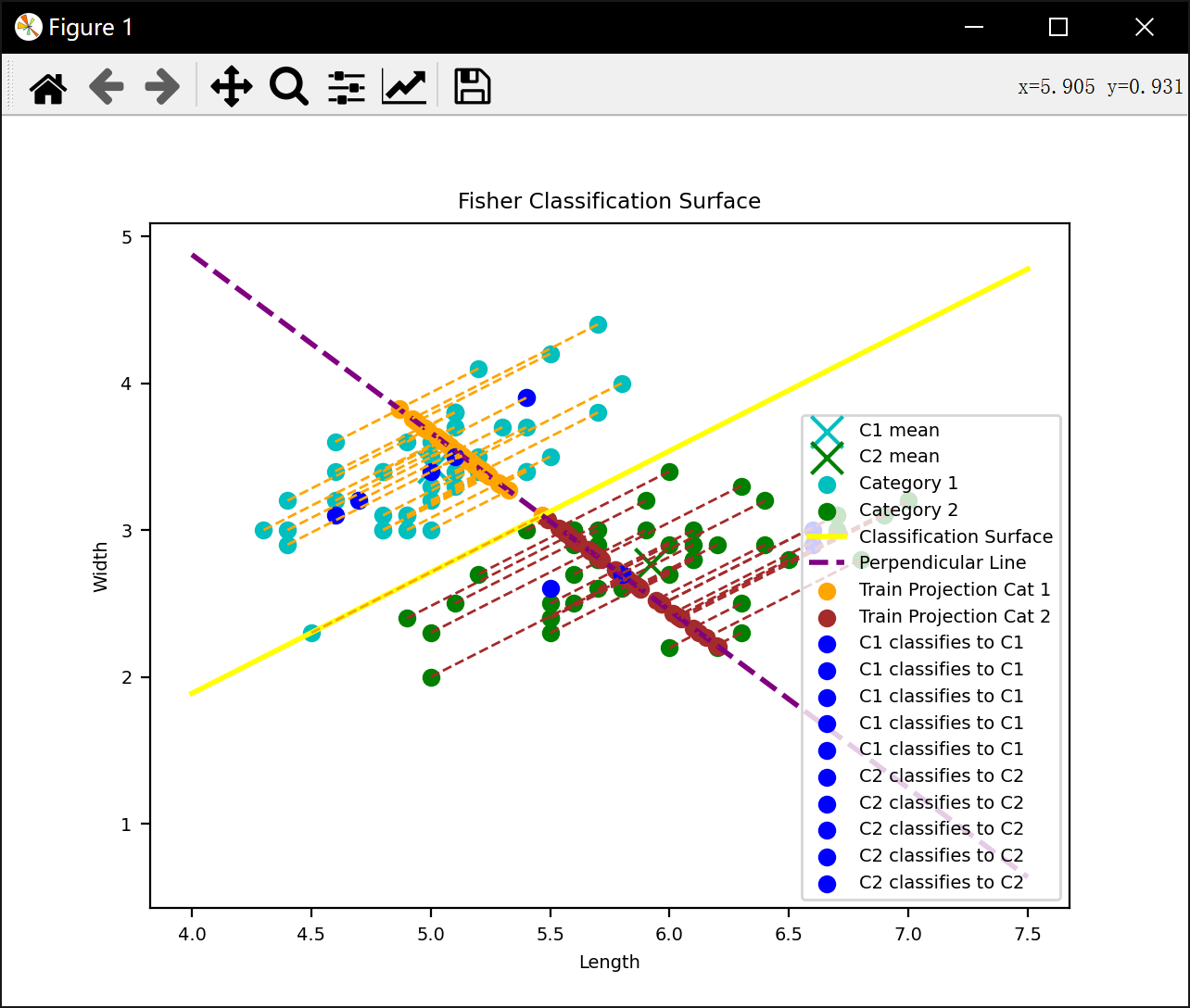
Fisher LDA:通过最大化类间散度与类内散度的比值,找到最优投影方向(分类超平面)。
-
分类决策:计算测试样本到分类超平面的距离,根据符号判断类别。
程序代码:
python
import random
import matplotlib
import matplotlib.pyplot as plt
import numpy as np

data_dict = {}
train_data = {}
test_data = {}

matplotlib.rcParams.update({'font.size': 7})

with open('Iris数据txt版.txt', 'r') as file:
    for line in file:
        line = line.strip()
        data = line.split('\t')
        if len(data) >= 3:
            try:
                category = data[0]
                attribute1 = eval(data[1])
                attribute2 = eval(data[2])
                if category in ['1', '2']:
                    if category not in data_dict:
                        data_dict[category] = {'Length': [], 'Width': []}

                    data_dict[category]['Length'].append(attribute1)
                    data_dict[category]['Width'].append(attribute2)
            except ValueError:
                print(f"Invalid data in line: {line}")
                continue
for category, attributes in data_dict.items():
    print(f'种类: {category}')
    print(len(attributes["Length"]))
    print(len(attributes["Width"]))
    print(f'属性1: {attributes["Length"]}')
    print(f'属性2: {attributes["Width"]}')

for category, attributes in data_dict.items():
    lengths = attributes['Length']
    widths = attributes['Width']
    train_indices = random.sample(range(len(lengths)), 45)
    test_indices = [i for i in range(len(lengths)) if i not in train_indices]

    train_data[category] = {
        'Length': [lengths[i] for i in train_indices],
        'Width': [widths[i] for i in train_indices]
    }

    test_data[category] = {
        'Length': [lengths[i] for i in test_indices],
        'Width': [widths[i] for i in test_indices]
    }

print(len(train_data['1']['Length']))
print(train_data['1'])
print(len(test_data['1']['Length']))
print(test_data['1'])
print(len(train_data['2']['Length']))
print(train_data['2'])
print(len(test_data['2']['Length']))
print(test_data['2'])

prior_rate = 1.0/len(data_dict)

#计算各个类中均值点和类间中值点
c1_mean = np.array([np.mean(train_data['1']['Length']), np.mean(train_data['1']['Width'])])
c2_mean = np.array([np.mean(train_data['2']['Length']), np.mean(train_data['2']['Width'])])
mean_diff = c2_mean - c1_mean
print("mean1",c1_mean.transpose())
print("mean2",c2_mean.transpose())
print("mean_diff",mean_diff)
middle_point = 0.5*(c1_mean+c2_mean)

#计算类内散度矩阵S1和S2
S1 = np.zeros((2, 2))
S2 = np.zeros((2, 2))

#计算分类面和投影面的参数a
for i in range(len(train_data['1']['Length'])):
    diff = np.array([train_data['1']['Length'][i] - c1_mean[0], train_data['1']['Width'][i] - c1_mean[1]])
    S1 += np.outer(diff, diff)

for i in range(len(train_data['2']['Length'])):
    diff = np.array([train_data['2']['Length'][i] - c2_mean[0], train_data['2']['Width'][i] - c2_mean[1]])
    S2 += np.outer(diff, diff)

print("S1",S1)
print("S2",S2)

#计算分类面和投影面的参数a
Sw = 0.5 * (S1 + S2)
a = np.linalg.inv(Sw).dot(mean_diff)
print("a", a)
b = -0.5 * (c1_mean + c2_mean).dot(a)
print("b", b)
slope_classification_line = -a[0] / a[1]
slope_vertical_line = -1 / slope_classification_line

#计算分类面和投影面的参数b
b_classification_line = -slope_classification_line * middle_point[0] + middle_point[1]
b_vertical_line = -slope_vertical_line * middle_point[0] + middle_point[1]

# 计算训练集的所有点到垂直分类面的投影点
train_projection_points_cat1 = []
train_projection_points_cat2 = []

for length, width in zip(train_data['1']['Length'], train_data['1']['Width']):
    bf = width - length*slope_classification_line
    projected_x_vertical = (bf-b_vertical_line)/(slope_vertical_line-slope_classification_line)
    projected_y_vertical = slope_vertical_line * projected_x_vertical + b_vertical_line

    train_projection_points_cat1.append([projected_x_vertical, projected_y_vertical])

for length, width in zip(train_data['2']['Length'], train_data['2']['Width']):
    bf = width - length * slope_classification_line
    projected_x_vertical = (bf - b_vertical_line) / (slope_vertical_line - slope_classification_line)
    projected_y_vertical = slope_vertical_line * projected_x_vertical + b_vertical_line

    train_projection_points_cat2.append([projected_x_vertical, projected_y_vertical])

train_projection_points_cat1 = np.array(train_projection_points_cat1)
train_projection_points_cat2 = np.array(train_projection_points_cat2)

#x的数据范围,分类面和垂直线的y值
x_range = np.linspace(4,7.5, 350)
y_range_classification_line = slope_classification_line * x_range + b_classification_line
y_range_vertical_line = slope_vertical_line * x_range + b_vertical_line

#画出训练数据点
plt.scatter(c1_mean[0], c1_mean[1], color='c', marker='x', s=150, label='C1 mean')
plt.scatter(c2_mean[0], c2_mean[1], color='g', marker='x', s=150, label='C2 mean')
plt.scatter(train_data['1']['Length'], train_data['1']['Width'], color='c', label='Category 1')
plt.scatter(train_data['2']['Length'], train_data['2']['Width'], color='g', label='Category 2')

#画出分类面和垂直线
plt.plot(x_range, y_range_classification_line, color='yellow', linewidth=2, label='Classification Surface')
plt.plot(x_range, y_range_vertical_line, color='purple', linestyle='dashed', linewidth=2, label='Perpendicular Line')

#画出训练数据点在投影线上的投影
plt.scatter(train_projection_points_cat1[:, 0], train_projection_points_cat1[:, 1], marker='o', color='orange', label='Train Projection Cat 1')
plt.scatter(train_projection_points_cat2[:, 0], train_projection_points_cat2[:, 1], marker='o', color='brown', label='Train Projection Cat 2')

#画出训练数据点到投影点的方向线
for i in range(len(train_projection_points_cat1)):
    plt.plot([train_data['1']['Length'][i], train_projection_points_cat1[i][0]],
             [train_data['1']['Width'][i], train_projection_points_cat1[i][1]], color='orange', linestyle='--', linewidth=1)

for i in range(len(train_projection_points_cat2)):
    plt.plot([train_data['2']['Length'][i], train_projection_points_cat2[i][0]],
             [train_data['2']['Width'][i], train_projection_points_cat2[i][1]], color='brown', linestyle='--', linewidth=1)

#将测试点分类并且输出结果,评估分类器性能
all = 0
right = 0

for length, width in zip(test_data['1']['Length'], test_data['1']['Width']):
    all += 1
    if slope_classification_line * length+b_classification_line - width < 0:
        plt.scatter(length, width, color='b',label= 'C1 classifies to C1')
        print("类别1数据 (", length, ",", width, ")分类到1,结果正确")
        right += 1
    elif slope_classification_line * length+b_classification_line - width > 0:
        plt.scatter(length, width, color='r',label= 'C1 classifies to C2')
        print("类别1数据 (", length, ",", width, ")分类到2,结果错误")
    else:
        plt.scatter(length, width, color='white',label= 'Unknown Classifier Result')
        print("类别1数据 (", length, ",", width, ")分类到分类面上,结果错误")

for length, width in zip(test_data['2']['Length'], test_data['2']['Width']):
    all += 1
    if slope_classification_line * length+b_classification_line - width > 0:
        plt.scatter(length, width, color='b',label= 'C2 classifies to C2')
        print("类别2数据 (", length, ",", width, ")分类到2,结果正确")
        right += 1
    elif slope_classification_line * length+b_classification_line - width < 0:
        plt.scatter(length, width, color='r',label= 'C1 classifies to C2')
        print("类别2数据 (", length, ",", width, ")分类到2,结果错误")
    else:
        plt.scatter(length, width, color='white',label= 'Unknown Classifier Result')
        print("类别2数据 (", length, ",", width, ")分类到分类面上,结果错误")

print("正确率:",right/all)
#画出图像结果
plt.xlabel('Length')
plt.ylabel('Width')
plt.legend()
plt.title('Fisher Classification Surface')
plt.show()
运行结果:
种类: 1
50
50
属性1: 5.1, 4.9, 4.7, 4.6, 5.0, 5.4, 4.6, 5.0, 4.4, 4.9, 5.4, 4.8, 4.8, 4.3, 5.8, 5.7, 5.4, 5.1, 5.7, 5.1, 5.4, 5.1, 4.6, 5.1, 4.8, 5.0, 5.0, 5.2, 5.2, 4.7, 4.8, 5.4, 5.2, 5.5, 4.9, 5.0, 5.5, 4.9, 4.4, 5.1, 5.0, 4.5, 4.4, 5.0, 5.1, 4.8, 5.1, 4.6, 5.3, 5.0
属性2: 3.5, 3.0, 3.2, 3.1, 3.6, 3.9, 3.4, 3.4, 2.9, 3.1, 3.7, 3.4, 3.0, 3.0, 4.0, 4.4, 3.9, 3.5, 3.8, 3.8, 3.4, 3.7, 3.6, 3.3, 3.4, 3.0, 3.4, 3.5, 3.4, 3.2, 3.1, 3.4, 4.1, 4.2, 3.1, 3.2, 3.5, 3.6, 3.0, 3.4, 3.5, 2.3, 3.2, 3.5, 3.8, 3.0, 3.8, 3.2, 3.7, 3.3
种类: 2
50
50
属性1: 7.0, 6.4, 6.9, 5.5, 6.5, 5.7, 6.3, 4.9, 6.6, 5.2, 5.0, 5.9, 6.0, 6.1, 5.6, 6.7, 5.6, 5.8, 6.2, 5.6, 5.9, 6.1, 6.3, 6.1, 6.4, 6.6, 6.8, 6.7, 6.0, 5.7, 5.5, 5.5, 5.8, 6.0, 5.4, 6.0, 6.7, 6.3, 5.6, 5.5, 5.5, 6.1, 5.8, 5.0, 5.6, 5.7, 5.7, 6.2, 5.1, 5.7
属性2: 3.2, 3.2, 3.1, 2.3, 2.8, 2.8, 3.3, 2.4, 2.9, 2.7, 2.0, 3.0, 2.2, 2.9, 2.9, 3.1, 3.0, 2.7, 2.2, 2.5, 3.2, 2.8, 2.5, 2.8, 2.9, 3.0, 2.8, 3.0, 2.9, 2.6, 2.4, 2.4, 2.7, 2.7, 3.0, 3.4, 3.1, 2.3, 3, 2.5, 2.6, 3.0, 2.6, 2.3, 2.7, 3.0, 2.9, 2.9, 2.5, 2.8
45
{'Length': 4.8, 4.6, 5.5, 5.0, 5.2, 4.8, 5.1, 4.9, 5.2, 5.4, 4.5, 4.4, 5.4, 5.0, 5.1, 4.7, 4.9, 5.4, 5.2, 4.8, 4.8, 5.0, 5.7, 5.3, 4.6, 5.0, 4.6, 4.4, 5.1, 5.4, 5.1, 4.9, 5.0, 5.1, 4.8, 5.8, 5.5, 5.1, 4.4, 5.1, 5.0, 4.3, 5.0, 4.9, 5.7, 'Width': 3.1, 3.6, 4.2, 3.2, 3.4, 3.0, 3.3, 3.1, 3.5, 3.7, 2.3, 3.0, 3.4, 3.5, 3.5, 3.2, 3.0, 3.9, 4.1, 3.0, 3.4, 3.4, 4.4, 3.7, 3.4, 3.3, 3.2, 2.9, 3.7, 3.4, 3.8, 3.6, 3.5, 3.4, 3.4, 4.0, 3.5, 3.8, 3.2, 3.8, 3.6, 3.0, 3.0, 3.1, 3.8}
5
{'Length': 4.6, 5.0, 5.4, 5.1, 4.7, 'Width': 3.1, 3.4, 3.9, 3.5, 3.2}
45
{'Length': 5.6, 7.0, 6.1, 4.9, 5.9, 5.5, 5.7, 6.7, 6.3, 5.6, 5.4, 6.2, 5.5, 5.7, 6.3, 5.2, 6.7, 6.4, 5.8, 6.1, 5.5, 6.1, 6.0, 6.0, 5.9, 5.0, 6.8, 6.0, 5.7, 6.5, 6.9, 6.0, 5.6, 5.6, 6.4, 5.1, 5.5, 6.2, 6.7, 5.7, 5.6, 5.7, 6.1, 5.0, 6.3, 'Width': 3, 3.2, 3.0, 2.4, 3.0, 2.4, 2.8, 3.1, 2.3, 2.9, 3.0, 2.9, 2.4, 2.8, 3.3, 2.7, 3.1, 2.9, 2.6, 2.8, 2.5, 2.8, 2.7, 2.9, 3.2, 2.3, 2.8, 3.4, 3.0, 2.8, 3.1, 2.2, 3.0, 2.7, 3.2, 2.5, 2.3, 2.2, 3.0, 2.6, 2.5, 2.9, 2.9, 2.0, 2.5}
5
{'Length': 6.6, 5.8, 6.6, 5.8, 5.5, 'Width': 2.9, 2.7, 3.0, 2.7, 2.6}
mean1 5.01111111 3.42888889
mean2 5.92222222 2.76888889
mean_diff 0.91111111 -0.66
S1 \[5.66444444 4.46555556
4.46555556 6.65244444\]
S2 \[11.93777778 3.84111111
3.84111111 4.71644444\]
a 0.24162727 -0.29265104
b -0.41400267302499916
类别1数据 ( 4.6 , 3.1 )分类到1,结果正确
类别1数据 ( 5.0 , 3.4 )分类到1,结果正确
类别1数据 ( 5.4 , 3.9 )分类到1,结果正确
类别1数据 ( 5.1 , 3.5 )分类到1,结果正确
类别1数据 ( 4.7 , 3.2 )分类到1,结果正确
类别2数据 ( 6.6 , 2.9 )分类到2,结果正确
类别2数据 ( 5.8 , 2.7 )分类到2,结果正确
类别2数据 ( 6.6 , 3.0 )分类到2,结果正确
类别2数据 ( 5.8 , 2.7 )分类到2,结果正确
类别2数据 ( 5.5 , 2.6 )分类到2,结果正确
正确率: 1.0