PBR学习笔记与Three.js中MeshPhysicalMaterial源码阅读

前言

PBR，全称Physically Based Rendering，翻译为基于物理的渲染技术，是遵循现实世界的物理规律的渲染技术，相比于基于经验的模型，PBR在一定程度上是物理正确的，所以在真实感上更加出色。在SIGGRAPH 2012上，迪士尼提出了著名的Disney Principled BRDF之后，PBR有了统一的标准，而且这一标准简单易用，简化了PBR的制作流程，被很多三维引擎和软件使用，如Unity, Unreal、3D Studio Max等。

Three.js也提供了PBR渲染技术，那就是MeshStandardMaterial和MeshPhysicalMaterial两个材质类。相比于基于经验模型的MeshLambertMaterial或MeshPhongMaterial等材质，基于PBR技术的材质在真实感上确实有很大的提升。

虽然说PBR标准确实简单易用，是对设计师友好的一套标准，但对于我们程序员来说，我们看待一个技术应该尽力做到知其然并知其所以然，如果可以理解背后的原理，就可以更灵活、更准确的使用这项技术，所以学习PBR的原理和阅读源码是非常有必要的。本文就是我学习和阅读源码的笔记。

在阅读MeshPhysicalMaterial类的源码时，为了降低难度和知识量，做了一定的简化。首先，本文只涉及不透明物体，不涉及非透明物体，考虑到多数物体都可以看做是非透明的，在一般的场景下也算够用。其次，本文阅读的过程中只涉及最常用的直射光DirectionalLight下的渲染。最后，本文只考虑直接光照下的渲染，不考虑间接光照。

光与物质表面的交互

既然是基于物理的渲染，那么这一节就介绍一下在真实的物理世界中，光和物质是如何交互的。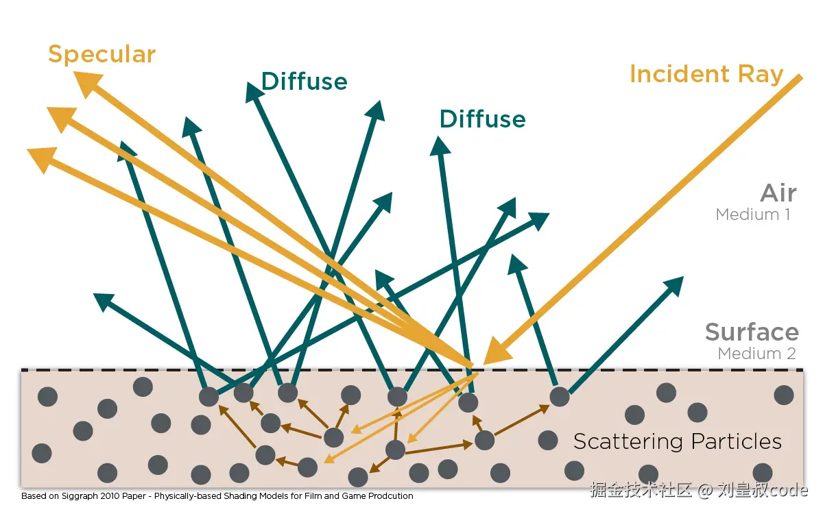

一束光入射到物体表面时，一部分光被物体表面反射（Reflection），反射的方向将遵循几何光学的规律，也就是镜面反射 （Specular）。一部分光则发生折射（Refraction），进入物体。进入物体的光会发生吸收（Absorption）和散射（Scattering）。物体的颜色一般是由于吸收不同波长的光引起的。对于不同的观察尺度来说，如果观察像素大于散射距离，散射被视为漫反射 （Diffuse），如果观察像素小于散射距离，散射被视为次表面散射 （Subsurface Scattering）。

根据材质的光学性质，一般将物体分为金属和非金属两类：

金属（Metal）：金属的外观主要取决于光线在两种介质的交界面上的直接反射,即镜面反射。折射入金属内部的光线几乎立即全部被自由电子吸收，所以射入金属的光不存在散射。
非金属 （No-Metal）：非金属也称电介质，入射到非金属的表面的光会分为反射和折射两部分。而折射的光又可以分为吸收和散射两部分。
总结来说，金属只需要考虑颜色和界面的反射；而非金属既要考虑反射，也要考虑折射。

微平面理论

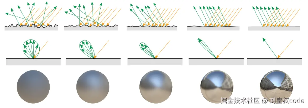
绝大多数真实世界的表面在微观尺度上都不是完全光滑的，而是有很多个微小的平面组成的，宏观上光入射到物体表面上产生的反射可以看做是光在这些微小平面上的镜面反射。微小平面的表面法线相对宏观上的表面法线有一定的偏差，这种偏差越是无序，从宏观上来看表面就越粗糙，所以物体材质有粗糙度 （roughness）这一属性。粗糙度 就是描述微小平面的法线分布与宏观上法线之间偏移程度的属性。粗糙度越大，反射光就越发散，表面就越模糊；反之，粗糙越小，反射光越趋向于同一方向，表面就越锐利。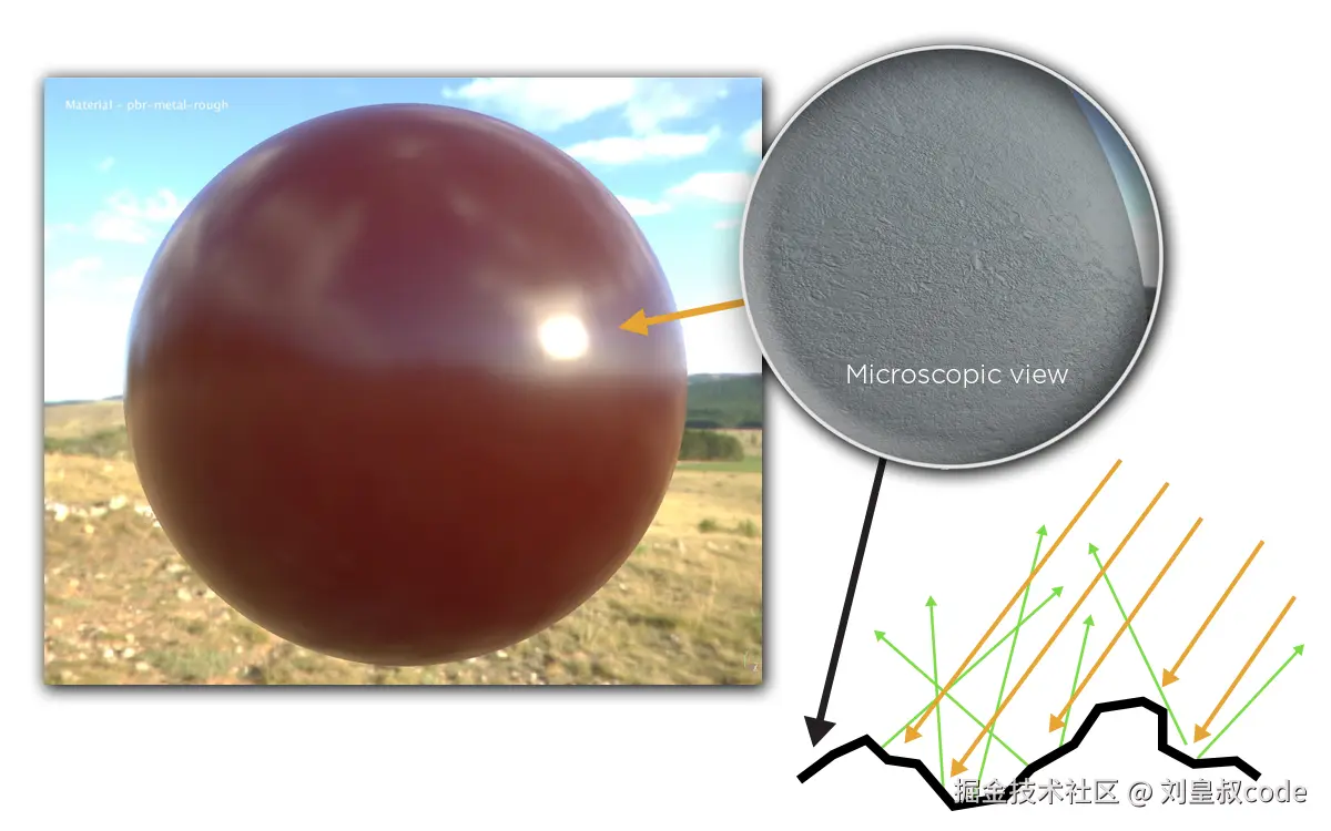

菲涅尔反射

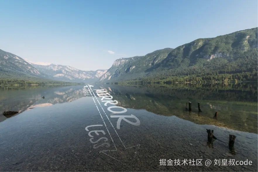
菲涅尔效应（Fresnel effect）表示的是物体表面反射光的程度取决于观察方向的现象。观察方向越靠近掠射角（与法线呈90度），光线越多，也就是反射率越大（如下图）。这个反射率就称为菲涅尔反射率。

物理上的菲涅尔方程比较复杂，这里不展示了。在实时渲染中一般使用Schlick近似来求菲涅尔反射率：
<math xmlns="http://www.w3.org/1998/Math/MathML" display="block"> F S c h l i c k ( h , v , F 0 ) = F 0 + ( 1 − F 0 ) ( 1 − ( v ⋅ h ) ) 5 F_{Schlick}(h,v,F_0)=F_0+(1-F_0)(1-(v \cdot h))^5 </math>FSchlick(h,v,F0)=F0+(1−F0)(1−(v⋅h))5

<math xmlns="http://www.w3.org/1998/Math/MathML"> F 0 F_0 </math>F0：物体表面的基础反射率，也就是光垂直表面入射时的反射率。
<math xmlns="http://www.w3.org/1998/Math/MathML"> v v </math>v：表示观察方向的向量。
<math xmlns="http://www.w3.org/1998/Math/MathML"> h h </math>h：观察方向与出射方向中间的向量，称为半角向量（half vector）。 <math xmlns="http://www.w3.org/1998/Math/MathML"> h = n o r m a l i z e ( ‌ l + v ) h=normalize(‌l+v) </math>h=normalize(‌l+v)。 <math xmlns="http://www.w3.org/1998/Math/MathML"> l l </math>l是光的入射方向的向量。

<math xmlns="http://www.w3.org/1998/Math/MathML"> F 0 F_0 </math>F0与折射率介质折射率之间的关系为：
<math xmlns="http://www.w3.org/1998/Math/MathML" display="block"> F 0 = ( n 1 − n 2 n 1 + n 2 ) 2 F_0=(\frac{n_1-n_2}{n_1+n_2})^2 </math>F0=(n1+n2n1−n2)2

其中 <math xmlns="http://www.w3.org/1998/Math/MathML"> n 1 n_1 </math>n1， <math xmlns="http://www.w3.org/1998/Math/MathML"> n 2 n_2 </math>n2是两种介质的折射率，考虑到绝大多数场景中，都是从空气入射到其他介质的，空气的折射率接近1，所以上式可以写作：
<math xmlns="http://www.w3.org/1998/Math/MathML" display="block"> F 0 = ( n − 1 n + 1 ) 2 F_0=(\frac{n-1}{n+1})^2 </math>F0=(n+1n−1)2

Disney Principled BRDF着色模型

本来在介绍BRDF之前，应该先介绍下渲染方程，但是考虑到这篇学习笔记性质的文章的篇幅已经比较长了，这里就不介绍了。不了解的同学可以去看我关于LightProbe的文章，其中简单介绍了下渲染方程，也可以看其他大佬比较详细文章。接下来介绍Disney Principled BRDF相关的内容，这里我没有将Disney Principled BRDF的发展历史和推导过程非常详尽的列出，而是只关注Three.js的MeshPhysicalMaterial类的代码用到的相关内容，对于Disney Principled BRDF发展历史和每一项的详细推导感兴趣的同学，可以去看这两位大佬的文章：
图形渲染基础：微表面材质模型
 【基于物理的渲染（PBR）白皮书】（三）迪士尼原则的BRDF与BSDF相关总结 Disney采用通用的microfacet Cook-Torrance BRDF着色模型：
<math xmlns="http://www.w3.org/1998/Math/MathML" display="block"> f ( l , v ) = d i f f u s e + D ( h ) F ( h , v ) G ( l , v ) 4 ( n ⋅ v ) ( n ⋅ l ) f(l,v)=diffuse+\frac{D(h)F(h,v)G(l,v)}{4(n \cdot v)(n \cdot l)} </math>f(l,v)=diffuse+4(n⋅v)(n⋅l)D(h)F(h,v)G(l,v)

diffuse为漫反射项，也就是非金属散射光引起的。
<math xmlns="http://www.w3.org/1998/Math/MathML"> D ( h ) F ( h , v ) G ( l , v ) 4 ( n ⋅ v ) ( n ⋅ l ) \frac{D(h)F(h,v)G(l,v)}{4(n \cdot v)(n \cdot l)} </math>4(n⋅v)(n⋅l)D(h)F(h,v)G(l,v)为镜面反射项，其中：
D为微平面法线分布函数。
F为菲涅尔反射系数。
G为几何衰减项。

漫反射项（Diffuse）

MeshPhysicalMaterial类的漫反射模型采用Lambert漫反射模型，Lambert模型假设折射光重新从入射表面发出时是均匀分布的，因此是一个常值函数。兰伯特模型没有方向性，也即它与入射光方向和观察方向无关。漫反射项只针对非金属材质，金属材质没有漫反射项。Lambert模型的表达式为：
<math xmlns="http://www.w3.org/1998/Math/MathML" display="block"> f l a m b e r t = ρ π f_{lambert}=\frac{\rho}{\pi} </math>flambert=πρ

<math xmlns="http://www.w3.org/1998/Math/MathML"> ρ \rho </math>ρ为漫反射的基础颜色。

微平面法线分布函数（NDF）

微平面的法线分布函数 <math xmlns="http://www.w3.org/1998/Math/MathML"> D ( m ) D(m) </math>D(m)描述了微观表面上的表面法线 <math xmlns="http://www.w3.org/1998/Math/MathML"> m m </math>m的统计分布。这个函数的值代表的是在一小块的宏观区域内，朝向以向量 <math xmlns="http://www.w3.org/1998/Math/MathML"> m m </math>m为中心的单位立体角 <math xmlns="http://www.w3.org/1998/Math/MathML"> ω m A m \omega_mAm </math>ωmAm的微平面的面积 <math xmlns="http://www.w3.org/1998/Math/MathML"> d A h dA_h </math>dAh与宏观区域面积 <math xmlns="http://www.w3.org/1998/Math/MathML"> A A </math>A的比值,所以NDF本质还是一个密度分布函数。有：
<math xmlns="http://www.w3.org/1998/Math/MathML" display="block"> d A h = D ( m ) d ω m A dA_h=D(m)d\omega_mA </math>dAh=D(m)dωmA

将 <math xmlns="http://www.w3.org/1998/Math/MathML"> D ( m ) D(m) </math>D(m)在立体角上积分，得到所有微平面的面积与宏观区域面积的比值，这个比值是大于等于1的。将所有微平面投影到宏观区域上，积分值则为1。有：
<math xmlns="http://www.w3.org/1998/Math/MathML" display="block"> ∫ Ω D ( m ) d ω i ≥ 1 \int_ΩD(m)dω_i\geq1 </math>∫ΩD(m)dωi≥1
<math xmlns="http://www.w3.org/1998/Math/MathML" display="block"> ∫ Ω D ( m ) ( n ⋅ m ) d ω i = 1 \int_ΩD(m)(n \cdot m)dω_i=1 </math>∫ΩD(m)(n⋅m)dωi=1

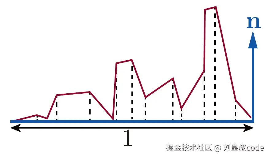法线越靠近宏观表面的法线的微平面，分布的面积越大，也就是说 <math xmlns="http://www.w3.org/1998/Math/MathML"> m m </math>m越靠近宏观表面的法线，NDF的值越大，在宏观表面的法线上，NDF达到峰值。

从宏观上来说，表面的粗糙度表示了微表面法线靠近宏观表面法线的程度，表面越粗糙，微表面法线越分散，反之则越集中。

一般来说，只有以半角向量 <math xmlns="http://www.w3.org/1998/Math/MathML"> h h </math>h为法线的微表面才能将光照反射到观察方向，而后被观察者看到，所以只有这部分微表面才对最终的渲染有贡献。

Disney Principled BRDF的法线分布选择Trowbridge-Reitz分布，又称为 GGX 分布。GGX的峰值比较窄，意味着GGX有更长的尾部。GGX的函数表达式为：
<math xmlns="http://www.w3.org/1998/Math/MathML" display="block"> D t r = α 2 π ( ( n ⋅ h ) 2 ( α 2 − 1 ) + 1 ) 2 D_{tr}=\frac{\alpha^2}{\pi((n \cdot h)^2(\alpha^2-1)+1)^2} </math>Dtr=π((n⋅h)2(α2−1)+1)2α2

<math xmlns="http://www.w3.org/1998/Math/MathML"> α \alpha </math>α代表表面粗糙度，值越大，代表表面越粗糙。

菲涅尔项（Specular F）

菲涅尔项上文已经介绍过了，采用Schlick近似来求得，这里不再赘述。在使用过程中， <math xmlns="http://www.w3.org/1998/Math/MathML"> F 0 F_0 </math>F0是一个三通道值，代表镜面反射的基础颜色的值。金属材质的所有可见颜色都由 <math xmlns="http://www.w3.org/1998/Math/MathML"> F 0 F_0 </math>F0决定。对于非金属来说，镜面反射颜色应该为单通道值，即R=G=B。但是在Disney Principled BRDF中为了对美术控制进行让步，还是提供了一个specularTint（非金属的镜面反射颜色）参数，所以在实际代码中非金属的 <math xmlns="http://www.w3.org/1998/Math/MathML"> F 0 F_0 </math>F0仍然是一个三通道值。

几何项（Specular G）

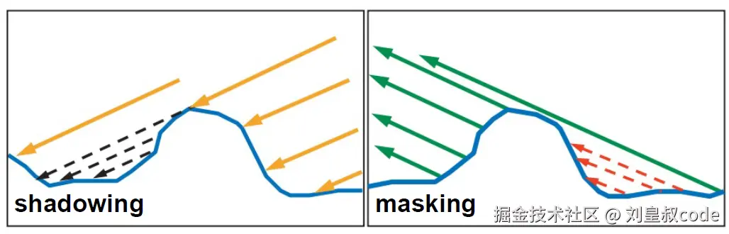
微表面实际上凹凸不平的，光线从光源入射到表面，并反射到观察方向的过程中，是有可能被凹凸不平的微表面挡住而不能最终被观察者接收到，几何项G就是用来描述这种能量损失的。

阴影（Shadowing）表示微平面对入射光的遮挡，一般是对光源方向而言。
遮蔽（masking）表示微平面对出射光的遮挡，一般是对观察方向而言。几何项G的发展经历了一个过程，推导过程也比较复杂，这里就不做介绍了，感兴趣的同学可以看这篇文章。【基于物理的渲染（PBR）白皮书】（五）几何函数相关总结
这里只列出MeshPhysicalMaterial中使用的GGX-Smith Correlated Joint Approximate方案：

<math xmlns="http://www.w3.org/1998/Math/MathML" display="block"> G ( l , v ) = 2 ( n ⋅ l ) ( n ⋅ v ) n ⋅ l ( n ⋅ v ) ( 1 − α 2 ) + α 2 + n ⋅ v ( n ⋅ l ) ( 1 − α 2 ) + α 2 G(l,v)=\frac{2(n \cdot l)(n \cdot v)}{n \cdot l\sqrt{(n \cdot v)(1 - \alpha^2)+\alpha^2}+n \cdot v\sqrt{(n \cdot l)(1 - \alpha^2)+\alpha^2}} </math>G(l,v)=n⋅l(n⋅v)(1−α2)+α2 +n⋅v(n⋅l)(1−α2)+α2 2(n⋅l)(n⋅v)

<math xmlns="http://www.w3.org/1998/Math/MathML"> α \alpha </math>α代表粗糙度。这个方案刚好可以和BRDF的分母消掉，可以写为：
<math xmlns="http://www.w3.org/1998/Math/MathML" display="block"> V ( l , v ) = 0.5 n ⋅ l ( n ⋅ v ) ( 1 − α 2 ) + α 2 + n ⋅ v ( n ⋅ l ) ( 1 − α 2 ) + α 2 V(l,v)=\frac{0.5}{n \cdot l\sqrt{(n \cdot v)(1 - \alpha^2)+\alpha^2}+n \cdot v\sqrt{(n \cdot l)(1 - \alpha^2)+\alpha^2}} </math>V(l,v)=n⋅l(n⋅v)(1−α2)+α2 +n⋅v(n⋅l)(1−α2)+α2 0.5

最终，镜面反射的BRDF可以写成：
<math xmlns="http://www.w3.org/1998/Math/MathML" display="block"> f s p e c u l a r = D ∗ F ∗ V f_{specular}=D*F*V </math>fspecular=D∗F∗V

MeshPhysicalMaterial类源码阅读

接下来我们一起来看下Three.js中MeshPhysicalMaterial的源码，我们重点关注的是直接光照的BRDF项是怎么计算的，与MeshPhysicalMaterial的各种属性之间的关系。首先我们来看lights_physical_fragment.glsl.js这段代码，这段代码主要是根据MeshPhysicalMaterial的属性来实例化一个结构体，并给这个结构体实例的成员赋值，以便后续计算BRDF。

glsl 复制代码

export default /* glsl */`
PhysicalMaterial material;
// metalnessFactor就是参数中的metalness与（如果有）采样的metalnessMap的b通道的乘积，就是金属度，
// 代表更偏向于金属的性质还是非金属。金属没有diffuse项，也就没有diffuseColor，diffuseColor就是参数中的diffuse。
material.diffuseColor = diffuseColor.rgb * ( 1.0 - metalnessFactor );

// 设置粗糙度，roughnessFactor就是参数中的roughness与（如果有）采样roughnessMap的g通道的乘积。
// 还增加了法线的变化率的影响。法线变化越剧烈就越粗糙。
vec3 dxy = max( abs( dFdx( nonPerturbedNormal ) ), abs( dFdy( nonPerturbedNormal ) ) );
float geometryRoughness = max( max( dxy.x, dxy.y ), dxy.z );

material.roughness = max( roughnessFactor, 0.0525 );// 0.0525 corresponds to the base mip of a 256 cubemap.
material.roughness += geometryRoughness;
material.roughness = min( material.roughness, 1.0 );

#ifdef IOR
    // 折射率，用来计算上文所说的F0
	material.ior = ior;

	#ifdef USE_SPECULAR
    // specularIntensity和specularColor，主要是对美术控制的妥协，允许为非金属设置高光反射颜色和反射强度，
    // 反射强度直接影响specularF90，用来计算菲涅尔项。
    // 对于金属来说，specularF90为1，specularColor就是diffuseColor，符合上文介绍的金属颜色全部来自反射。
		float specularIntensityFactor = specularIntensity;
		vec3 specularColorFactor = specularColor;

		#ifdef USE_SPECULAR_COLORMAP

			specularColorFactor *= texture2D( specularColorMap, vSpecularColorMapUv ).rgb;

		#endif

		#ifdef USE_SPECULAR_INTENSITYMAP

			specularIntensityFactor *= texture2D( specularIntensityMap, vSpecularIntensityMapUv ).a;

		#endif

		material.specularF90 = mix( specularIntensityFactor, 1.0, metalnessFactor );

	#else

		float specularIntensityFactor = 1.0;
		vec3 specularColorFactor = vec3( 1.0 );
		material.specularF90 = 1.0;

	#endif

	material.specularColor = mix( min( pow2( ( material.ior - 1.0 ) / ( material.ior + 1.0 ) ) * specularColorFactor, vec3( 1.0 ) ) * specularIntensityFactor, diffuseColor.rgb, metalnessFactor );

#else

	material.specularColor = mix( vec3( 0.04 ), diffuseColor.rgb, metalnessFactor );
	material.specularF90 = 1.0;

#endif

// 清漆层，在表面增加了一层镜面反射，可以让表面的镜面反射更加明显，后文会介绍。
//常见的清漆材质的f0近似为0.04，f90为1。
#ifdef USE_CLEARCOAT

	material.clearcoat = clearcoat;
	material.clearcoatRoughness = clearcoatRoughness;
	material.clearcoatF0 = vec3( 0.04 );
	material.clearcoatF90 = 1.0;

	#ifdef USE_CLEARCOATMAP

		material.clearcoat *= texture2D( clearcoatMap, vClearcoatMapUv ).x;

	#endif

	#ifdef USE_CLEARCOAT_ROUGHNESSMAP

		material.clearcoatRoughness *= texture2D( clearcoatRoughnessMap, vClearcoatRoughnessMapUv ).y;

	#endif

	material.clearcoat = saturate( material.clearcoat ); // Burley clearcoat model
	material.clearcoatRoughness = max( material.clearcoatRoughness, 0.0525 );
	material.clearcoatRoughness += geometryRoughness;
	material.clearcoatRoughness = min( material.clearcoatRoughness, 1.0 );

#endif

#ifdef USE_DISPERSION

	material.dispersion = dispersion;

#endif

#ifdef USE_IRIDESCENCE

	material.iridescence = iridescence;
	material.iridescenceIOR = iridescenceIOR;

	#ifdef USE_IRIDESCENCEMAP

		material.iridescence *= texture2D( iridescenceMap, vIridescenceMapUv ).r;

	#endif

	#ifdef USE_IRIDESCENCE_THICKNESSMAP

		material.iridescenceThickness = (iridescenceThicknessMaximum - iridescenceThicknessMinimum) * texture2D( iridescenceThicknessMap, vIridescenceThicknessMapUv ).g + iridescenceThicknessMinimum;

	#else

		material.iridescenceThickness = iridescenceThicknessMaximum;

	#endif

#endif

// 光泽度，主要用于模拟布料等材质，后文会介绍。
#ifdef USE_SHEEN

	material.sheenColor = sheenColor;

	#ifdef USE_SHEEN_COLORMAP

		material.sheenColor *= texture2D( sheenColorMap, vSheenColorMapUv ).rgb;

	#endif

	material.sheenRoughness = clamp( sheenRoughness, 0.07, 1.0 );

	#ifdef USE_SHEEN_ROUGHNESSMAP

		material.sheenRoughness *= texture2D( sheenRoughnessMap, vSheenRoughnessMapUv ).a;

	#endif

#endif

//各项异性，用于控制镜面反射高光的纵横比，可以模拟类似金属拉丝工艺的材质，后文会介绍。
#ifdef USE_ANISOTROPY
	// anisotropyRotation与anisotropyMap（如果有）参数计算anisotropyVector
	#ifdef USE_ANISOTROPYMAP

		mat2 anisotropyMat = mat2( anisotropyVector.x, anisotropyVector.y, - anisotropyVector.y, anisotropyVector.x );
		vec3 anisotropyPolar = texture2D( anisotropyMap, vAnisotropyMapUv ).rgb;
		vec2 anisotropyV = anisotropyMat * normalize( 2.0 * anisotropyPolar.rg - vec2( 1.0 ) ) * anisotropyPolar.b;

	#else

		vec2 anisotropyV = anisotropyVector;

	#endif

	material.anisotropy = length( anisotropyV );

	if( material.anisotropy == 0.0 ) {
		anisotropyV = vec2( 1.0, 0.0 );
	} else {
		anisotropyV /= material.anisotropy;
		material.anisotropy = saturate( material.anisotropy );
	}

	// Roughness along the anisotropy bitangent is the material roughness, while the tangent roughness increases with anisotropy.
	material.alphaT = mix( pow2( material.roughness ), 1.0, pow2( material.anisotropy ) );
	// 将anisotropyVector转换到世界坐标系中，就是切线方向和副切线方向。
	material.anisotropyT = tbn[ 0 ] * anisotropyV.x + tbn[ 1 ] * anisotropyV.y;
	material.anisotropyB = tbn[ 1 ] * anisotropyV.x - tbn[ 0 ] * anisotropyV.y;

#endif
`;

接下来是RE_Direct_Physical这个函数了，这个函数是直射光依据渲染方程计算每一点的直接光照的渲染结果的。

glsl 复制代码

void RE_Direct_Physical( const in IncidentLight directLight, const in vec3 geometryPosition, const in vec3 geometryNormal, const in vec3 geometryViewDir, const in vec3 geometryClearcoatNormal, const in PhysicalMaterial material, inout ReflectedLight reflectedLight ) {

    //ωi·n,入射方向和法向量的点乘
	float dotNL = saturate( dot( geometryNormal, directLight.direction ) );
	//光照颜色乘cosΘ，就是这个点接收的irradiance
	vec3 irradiance = dotNL * directLight.color;
	//如果有clearcoat，计算清漆层的镜面反射结果
	#ifdef USE_CLEARCOAT

		float dotNLcc = saturate( dot( geometryClearcoatNormal, directLight.direction ) );

		vec3 ccIrradiance = dotNLcc * directLight.color;

		clearcoatSpecularDirect += ccIrradiance * BRDF_GGX_Clearcoat( directLight.direction, geometryViewDir, geometryClearcoatNormal, material );

	#endif
	//如果有sheen，计算sheen的镜面反射结果
	#ifdef USE_SHEEN

		sheenSpecularDirect += irradiance * BRDF_Sheen( directLight.direction, geometryViewDir, geometryNormal, material.sheenColor, material.sheenRoughness );

	#endif

	//irradiance乘GGX分布的BRDF就是镜面反射结果
	reflectedLight.directSpecular += irradiance * BRDF_GGX( directLight.direction, geometryViewDir, geometryNormal, material );
	//irradiance乘Lambert模型的BRDF就是镜面反射结果
	reflectedLight.directDiffuse += irradiance * BRDF_Lambert( material.diffuseColor );
}

下面就是计算BRDF项了，这里对roughness求了平方，这是因为用户设定的粗糙度为感知粗糙度，求平方将其重新映射到感知线性范围，这更容易被美术和开发人员理解，如果不使用映射，光泽金属表面的值必须限制在0到0.05之间的非常小的范围。

glsl 复制代码

vec3 BRDF_GGX( const in vec3 lightDir, const in vec3 viewDir, const in vec3 normal, const in PhysicalMaterial material ) {
    // f0表示基础的镜面反射颜色，也就是正对微表面时的镜面颜色
	vec3 f0 = material.specularColor;
    //f90表示掠射角镜面反射强度，对于金属材质来说是1，对于非金属可以手动设置。
	float f90 = material.specularF90;
    // 粗糙度，对于法线分布项和几何项都有影响。
	float roughness = material.roughness;

	float alpha = pow2( roughness ); // UE4's roughness

	vec3 halfDir = normalize( lightDir + viewDir );
    //入射方向和宏观法线方向的点乘
	float dotNL = saturate( dot( normal, lightDir ) );
    //观察方向和宏观法线方向的点乘
	float dotNV = saturate( dot( normal, viewDir ) );
    //半角向量和宏观法线方向的点乘
	float dotNH = saturate( dot( normal, halfDir ) );
    //观察方向和半角向量的点乘
	float dotVH = saturate( dot( viewDir, halfDir ) );
    //计算菲涅尔项
	vec3 F = F_Schlick( f0, f90, dotVH );

	#ifdef USE_IRIDESCENCE

		F = mix( F, material.iridescenceFresnel, material.iridescence );

	#endif
    //各向异性，如果材质为各向异性，会替换各向同性的法线分布项和几何项，具体原理后文介绍。
	#ifdef USE_ANISOTROPY

		float dotTL = dot( material.anisotropyT, lightDir );
		float dotTV = dot( material.anisotropyT, viewDir );
		float dotTH = dot( material.anisotropyT, halfDir );
		float dotBL = dot( material.anisotropyB, lightDir );
		float dotBV = dot( material.anisotropyB, viewDir );
		float dotBH = dot( material.anisotropyB, halfDir );

		float V = V_GGX_SmithCorrelated_Anisotropic( material.alphaT, alpha, dotTV, dotBV, dotTL, dotBL, dotNV, dotNL );

		float D = D_GGX_Anisotropic( material.alphaT, alpha, dotNH, dotTH, dotBH );

	#else
        //计算几何项
		float V = V_GGX_SmithCorrelated( alpha, dotNL, dotNV );
        //计算法线分布项
		float D = D_GGX( alpha, dotNH );

	#endif
    //BRDF项就是菲涅尔项、几何项和法线分布项的乘积。
	return F * ( V * D );

}

下面是菲涅尔项、几何项和法线分布项的计算代码，和上文介绍的数学原理一致，就不多介绍了。

glsl 复制代码

vec3 F_Schlick( const in vec3 f0, const in float f90, const in float dotVH ) {

	// Original approximation by Christophe Schlick '94
	// float fresnel = pow( 1.0 - dotVH, 5.0 );

	// Optimized variant (presented by Epic at SIGGRAPH '13)
	// https://cdn2.unrealengine.com/Resources/files/2013SiggraphPresentationsNotes-26915738.pdf
	float fresnel = exp2( ( - 5.55473 * dotVH - 6.98316 ) * dotVH );

	return f0 * ( 1.0 - fresnel ) + ( f90 * fresnel );

}

glsl 复制代码

// Moving Frostbite to Physically Based Rendering 3.0 - page 12, listing 2
// https://seblagarde.files.wordpress.com/2015/07/course_notes_moving_frostbite_to_pbr_v32.pdf
float V_GGX_SmithCorrelated( const in float alpha, const in float dotNL, const in float dotNV ) {

	float a2 = pow2( alpha );

	float gv = dotNL * sqrt( a2 + ( 1.0 - a2 ) * pow2( dotNV ) );
	float gl = dotNV * sqrt( a2 + ( 1.0 - a2 ) * pow2( dotNL ) );

	return 0.5 / max( gv + gl, EPSILON );

}

glsl 复制代码

// Microfacet Models for Refraction through Rough Surfaces - equation (33)
// http://graphicrants.blogspot.com/2013/08/specular-brdf-reference.html
// alpha is "roughness squared" in Disney's reparameterization
float D_GGX( const in float alpha, const in float dotNH ) {

	float a2 = pow2( alpha );

	float denom = pow2( dotNH ) * ( a2 - 1.0 ) + 1.0; // avoid alpha = 0 with dotNH = 1

	return RECIPROCAL_PI * a2 / pow2( denom );

}

sheen

sheen相关参数主要针对布料等材质的渲染，如下图，左边是没有sheenColor,右边有sheenColor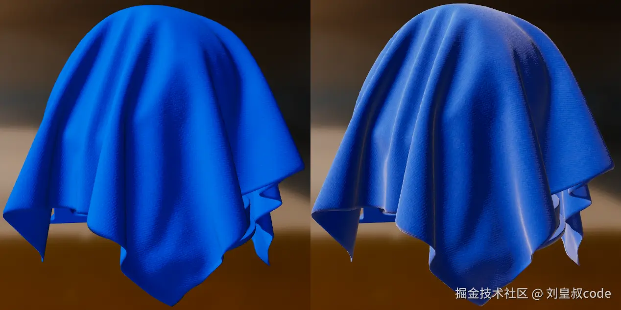： Three.js采用了计算成本较低，且有更柔和的外观的BRDF计算公式。法线分布函数NDF为：
<math xmlns="http://www.w3.org/1998/Math/MathML" display="block"> D ( m ) = ( 2 + 1 α ) ( sin ⁡ θ ) 1 α 2 π D(m)=\frac{(2+\frac{1}{\alpha})(\sin\theta)^\frac{1}{\alpha}}{2\pi} </math>D(m)=2π(2+α1)(sinθ)α1

完整的BRDF为：
<math xmlns="http://www.w3.org/1998/Math/MathML" display="block"> f r ( l , v , α ) = D ( h ) 4 ( n ⋅ v + n ⋅ l − ( n ⋅ v ) ( n ⋅ l ) ) f_r(l,v,\alpha)=\frac{D(h)}{4(n \cdot v+n \cdot l-(n \cdot v)(n \cdot l))} </math>fr(l,v,α)=4(n⋅v+n⋅l−(n⋅v)(n⋅l))D(h)

js 复制代码

float D_Charlie( float roughness, float dotNH ) {

	float alpha = pow2( roughness );

	// Estevez and Kulla 2017, "Production Friendly Microfacet Sheen BRDF"
	float invAlpha = 1.0 / alpha;
	float cos2h = dotNH * dotNH;
	float sin2h = max( 1.0 - cos2h, 0.0078125 ); // 2^(-14/2), so sin2h^2 > 0 in fp16

	return ( 2.0 + invAlpha ) * pow( sin2h, invAlpha * 0.5 ) / ( 2.0 * PI );

}

// https://github.com/google/filament/blob/master/shaders/src/brdf.fs
float V_Neubelt( float dotNV, float dotNL ) {

	// Neubelt and Pettineo 2013, "Crafting a Next-gen Material Pipeline for The Order: 1886"
	return saturate( 1.0 / ( 4.0 * ( dotNL + dotNV - dotNL * dotNV ) ) );

}

vec3 BRDF_Sheen( const in vec3 lightDir, const in vec3 viewDir, const in vec3 normal, vec3 sheenColor, const in float sheenRoughness ) {

	vec3 halfDir = normalize( lightDir + viewDir );

	float dotNL = saturate( dot( normal, lightDir ) );
	float dotNV = saturate( dot( normal, viewDir ) );
	float dotNH = saturate( dot( normal, halfDir ) );

	float D = D_Charlie( sheenRoughness, dotNH );
	float V = V_Neubelt( dotNV, dotNL );

	return sheenColor * ( D * V );

}

clearcoat

clearcoat（清漆）,效果就是在物体表面会涂上一层薄薄的非金属的透明层，比如汽车涂装、漆器。如下图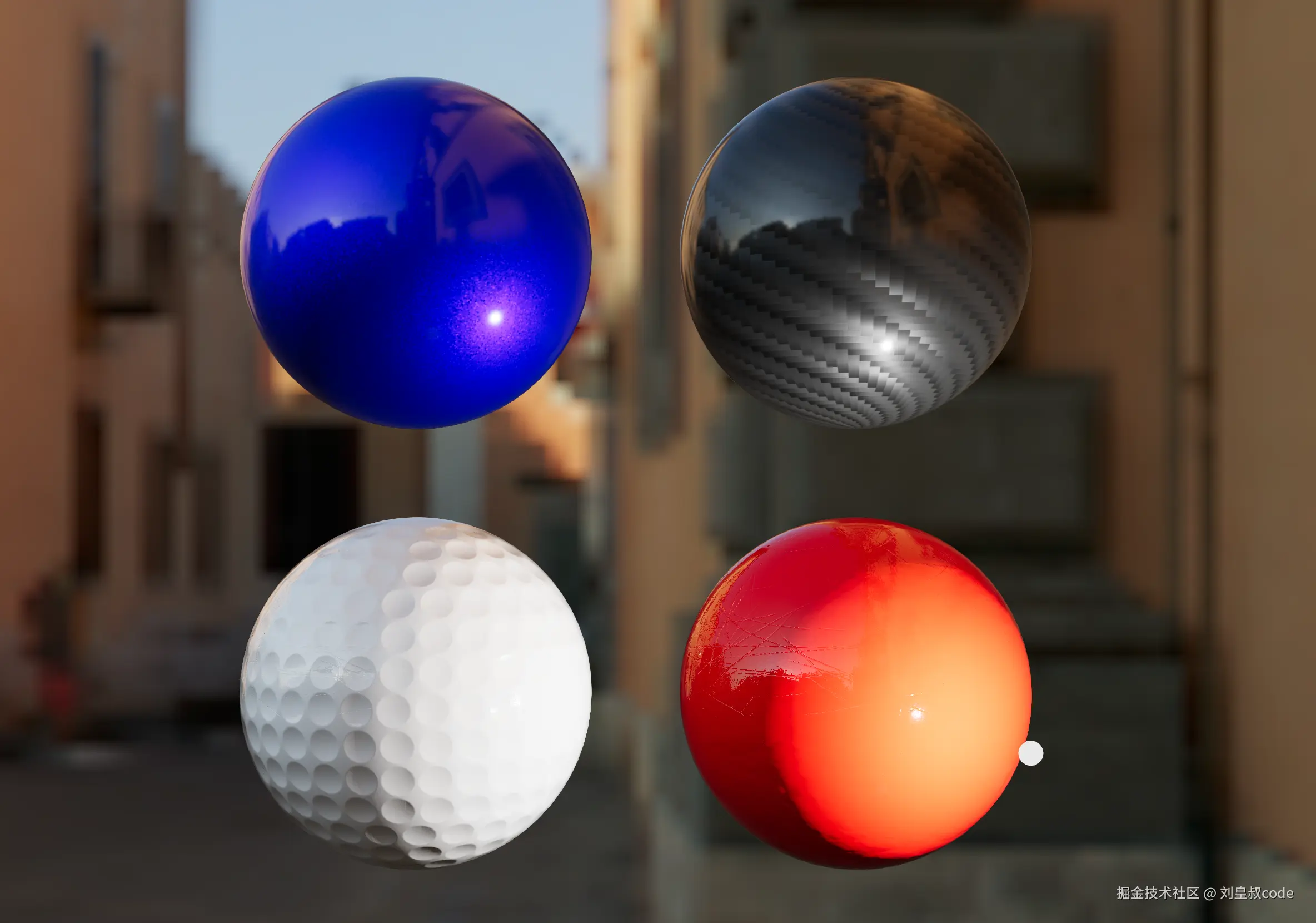：这是一种多层材质，并且清漆层总是各向同性的。清漆层是透明的，不考虑颜色，不考虑折射，也不考虑清漆层与基础层之间的反射，常见的清漆或涂料的 <math xmlns="http://www.w3.org/1998/Math/MathML"> f 0 f_0 </math>f0可以近似为0.04。可以用一个额外的镜面反射BRDF描述。代码如下：

glsl 复制代码

vec3 BRDF_GGX_Clearcoat( const in vec3 lightDir, const in vec3 viewDir, const in vec3 normal, const in PhysicalMaterial material) {
	//clearcoat的f0固定为vec3(0.04)
	vec3 f0 = material.clearcoatF0;
	//f90固定为1.0
	float f90 = material.clearcoatF90;
	float roughness = material.clearcoatRoughness;

	float alpha = pow2( roughness ); // UE4's roughness

	vec3 halfDir = normalize( lightDir + viewDir );

	float dotNL = saturate( dot( normal, lightDir ) );
	float dotNV = saturate( dot( normal, viewDir ) );
	float dotNH = saturate( dot( normal, halfDir ) );
	float dotVH = saturate( dot( viewDir, halfDir ) );

	vec3 F = F_Schlick( f0, f90, dotVH );

	float V = V_GGX_SmithCorrelated( alpha, dotNL, dotNV );

	float D = D_GGX( alpha, dotNH );

	return F * ( V * D );

}

anisotropy

现实中的很多材质的镜面反射，比如拉丝金属，需要各向异性模型的支持才能模拟。如下图，左边是各项同性，右边是各项异性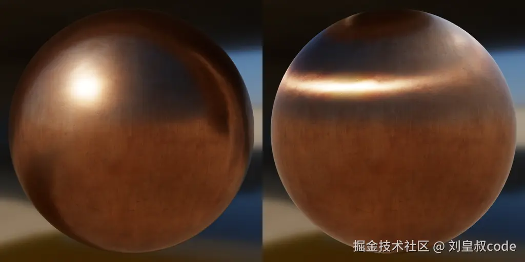：各向异性的BRDF可以在之前各向同性的基础上修改。GGX法线分布函数具体可以修改为：
<math xmlns="http://www.w3.org/1998/Math/MathML" display="block"> D a n i s o ( h , a ) = 1 π α t α b 1 [ ( t ⋅ h α t ) 2 + ( b ⋅ h α b ) 2 + ( n ⋅ h ) 2 ] 2 D_{aniso}(h,a)=\frac{1}{\pi\alpha_t\alpha_b}\frac{1}{[(\frac{t \cdot h}{\alpha_t})^2+(\frac{b \cdot h}{\alpha_b})^2+(n \cdot h)^2]^2} </math>Daniso(h,a)=παtαb1[(αtt⋅h)2+(αbb⋅h)2+(n⋅h)2]21

<math xmlns="http://www.w3.org/1998/Math/MathML"> t t </math>t和 <math xmlns="http://www.w3.org/1998/Math/MathML"> b b </math>b分别是切线方向向量和副切线方向向量， <math xmlns="http://www.w3.org/1998/Math/MathML"> α t \alpha_t </math>αt和 <math xmlns="http://www.w3.org/1998/Math/MathML"> α b \alpha_b </math>αb分别是切线方向和副切向方向的粗糙度。切线方向和副切线方向由MeshPhsicalMaterial中的anisotropyRotation或anisotropyMap参数决定。在Three.js中副切线的粗糙度为材质的粗糙度，切线的粗糙度会随着anisotropy参数的增大而增大，如下：
<math xmlns="http://www.w3.org/1998/Math/MathML" display="block"> α t = l e r p ( α , 1 , a n i s o t r o p y 2 ) \alpha_t=lerp(\alpha,1,anisotropy^2) </math>αt=lerp(α,1,anisotropy2)
<math xmlns="http://www.w3.org/1998/Math/MathML" display="block"> α b = α \alpha_b=\alpha </math>αb=α

几何项可以修改为：
<math xmlns="http://www.w3.org/1998/Math/MathML" display="block"> V a n i s o ( n ⋅ l , n ⋅ v , α ) = 1 2 [ ( n ⋅ l ) α t 2 ( t ⋅ v ) 2 + α b 2 ( b ⋅ v ) 2 + ( n ⋅ v ) 2 + ( n ⋅ l ) α t 2 ( t ⋅ l ) 2 + α b 2 ( b ⋅ l ) 2 + ( n ⋅ l ) 2 ] V_{aniso}(n \cdot l,n \cdot v,\alpha)=\frac{1}{2[(n \cdot l)\sqrt{\alpha_t^2(t \cdot v)^2+\alpha_b^2(b \cdot v)^2+(n \cdot v)^2}+(n \cdot l)\sqrt{\alpha_t^2(t \cdot l)^2+\alpha_b^2(b \cdot l)^2+(n \cdot l)^2}]} </math>Vaniso(n⋅l,n⋅v,α)=2[(n⋅l)αt2(t⋅v)2+αb2(b⋅v)2+(n⋅v)2 +(n⋅l)αt2(t⋅l)2+αb2(b⋅l)2+(n⋅l)2 ]1

代码如下：

js 复制代码

float V_GGX_SmithCorrelated_Anisotropic( const in float alphaT, const in float alphaB, const in float dotTV, const in float dotBV, const in float dotTL, const in float dotBL, const in float dotNV, const in float dotNL ) {

	float gv = dotNL * length( vec3( alphaT * dotTV, alphaB * dotBV, dotNV ) );
	float gl = dotNV * length( vec3( alphaT * dotTL, alphaB * dotBL, dotNL ) );
	float v = 0.5 / ( gv + gl );

	return saturate(v);

}

float D_GGX_Anisotropic( const in float alphaT, const in float alphaB, const in float dotNH, const in float dotTH, const in float dotBH ) {

	float a2 = alphaT * alphaB;
	highp vec3 v = vec3( alphaB * dotTH, alphaT * dotBH, a2 * dotNH );
	highp float v2 = dot( v, v );
	float w2 = a2 / v2;

	return RECIPROCAL_PI * a2 * pow2 ( w2 );

}

本文的初衷是因为在使用MeshPhysicalMaterial类时，对于其中的参数的意义不甚了解，所以就想通过学习PBR和阅读源码来加深理解。通过这个过程，对于color(diffuse)、metalness、roughness、specular、sheen、anisotropy、clearcoat等相关的参数的原理有了较为全面的理解。