EfficientNet模型:高效卷积神经网络的革命性突破
🌟 你好,我是 励志成为糕手 !
🌌 在代码的宇宙中,我是那个追逐优雅与性能的星际旅人。
✨ 每一行代码都是我种下的星光,在逻辑的土壤里生长成璀璨的银河;
🛠️ 每一个算法都是我绘制的星图,指引着数据流动的最短路径;
🔍 每一次调试都是星际对话,用耐心和智慧解开宇宙的谜题。
🚀 准备好开始我们的星际编码之旅了吗?
目录
- EfficientNet模型:高效卷积神经网络的革命性突破
-
- 摘要
- [1. EfficientNet核心原理](#1. EfficientNet核心原理)
-
- [1.1 复合缩放方法](#1.1 复合缩放方法)
- [1.2 缩放系数的数学原理](#1.2 缩放系数的数学原理)
- [2. MBConv模块架构](#2. MBConv模块架构)
-
- [2.1 移动倒置瓶颈卷积](#2.1 移动倒置瓶颈卷积)
- [2.2 MBConv模块实现](#2.2 MBConv模块实现)
- [3. EfficientNet完整架构](#3. EfficientNet完整架构)
-
- [3.1 网络架构设计](#3.1 网络架构设计)
- [3.2 完整网络实现](#3.2 完整网络实现)
- [4. 性能对比分析](#4. 性能对比分析)
-
- [4.1 不同模型性能对比](#4.1 不同模型性能对比)
- [4.2 效率分析图表](#4.2 效率分析图表)
- [5. 训练策略与优化](#5. 训练策略与优化)
-
- [5.1 渐进式训练策略](#5.1 渐进式训练策略)
- [5.2 数据增强策略](#5.2 数据增强策略)
- [6. 实际应用案例](#6. 实际应用案例)
-
- [6.1 图像分类任务](#6.1 图像分类任务)
- [6.2 迁移学习应用](#6.2 迁移学习应用)
- [7. 模型优化与部署](#7. 模型优化与部署)
-
- [7.1 模型量化](#7.1 模型量化)
- [7.2 模型部署优化](#7.2 模型部署优化)
- [8. 未来发展趋势](#8. 未来发展趋势)
-
- [8.1 EfficientNet演进路线](#8.1 EfficientNet演进路线)
- [8.2 技术发展预测](#8.2 技术发展预测)
- 总结
- 参考链接
- 关键词标签
摘要
作为一名深度学习的探索者,我在研究卷积神经网络的道路上遇到了一个令人兴奋的里程碑------EfficientNet。这个模型彻底改变了我对网络设计的认知,它不仅在ImageNet上刷新了准确率记录,更重要的是用更少的参数和计算量达到了前所未有的效果。
EfficientNet的核心思想让我深深着迷:通过复合缩放(Compound Scaling)方法,同时优化网络的深度、宽度和分辨率,而不是传统的单一维度扩展。这种设计哲学就像是在三维空间中寻找最优解,而不是在单一轴线上盲目前进。当我第一次看到EfficientNet-B7在ImageNet上达到84.4%的top-1准确率,同时参数量比GPipe少8.4倍时,我意识到这不仅仅是一个模型的改进,而是整个网络设计范式的革新。
在实际项目中,我发现EfficientNet的魅力远不止于此。它的MBConv(Mobile Inverted Bottleneck Convolution)模块巧妙地结合了深度可分离卷积和Squeeze-and-Excitation注意力机制,让每一层都能高效地提取特征。更令人惊喜的是,通过神经架构搜索(NAS)技术找到的基础架构EfficientNet-B0,为后续的缩放提供了坚实的基础。这种从B0到B7的系统性扩展,让我们可以根据不同的计算资源和精度需求,选择最适合的模型变体。
1. EfficientNet核心原理
1.1 复合缩放方法
EfficientNet最大的创新在于提出了复合缩放方法。传统的网络扩展通常只关注单一维度,要么增加深度,要么增加宽度,要么提高输入分辨率。但EfficientNet认为这三个维度应该协调发展。
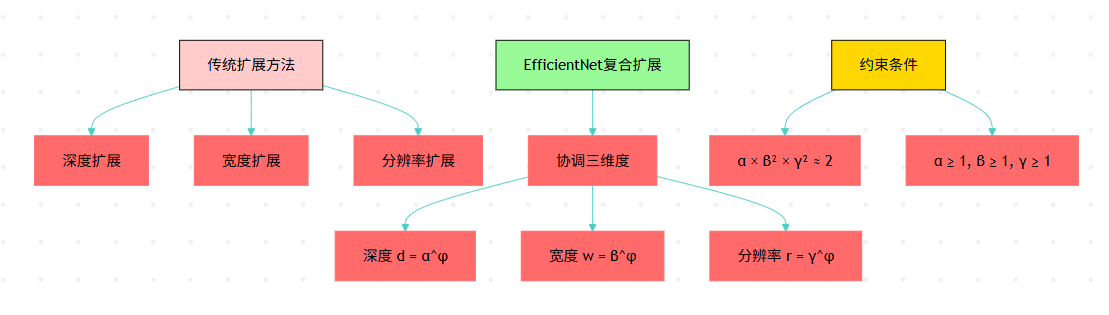
图1:EfficientNet复合缩放方法对比流程图
1.2 缩放系数的数学原理
复合缩放的核心公式非常优雅:
python
# EfficientNet复合缩放核心实现
import math

class CompoundScaling:
    def __init__(self, alpha=1.2, beta=1.1, gamma=1.15):
        """
        初始化复合缩放参数
        alpha: 深度缩放系数
        beta: 宽度缩放系数
        gamma: 分辨率缩放系数
        """
        self.alpha = alpha
        self.beta = beta
        self.gamma = gamma

        # 验证约束条件:α × β² × γ² ≈ 2
        constraint = alpha * (beta ** 2) * (gamma ** 2)
        print(f"约束条件验证: {constraint:.3f} ≈ 2.0")

    def scale_network(self, phi, base_depth=7, base_width=1.0, base_resolution=224):
        """
        根据复合系数φ缩放网络
        """
        # 计算缩放后的维度
        scaled_depth = math.ceil(self.alpha ** phi * base_depth)
        scaled_width = self.beta ** phi * base_width
        scaled_resolution = int(self.gamma ** phi * base_resolution)

        return {
            'depth': scaled_depth,
            'width': scaled_width,
            'resolution': scaled_resolution,
            'phi': phi
        }

# 演示不同EfficientNet变体的缩放
scaler = CompoundScaling()

# 生成B0到B7的配置
efficientnet_configs = {}
for i in range(8):
    config = scaler.scale_network(phi=i)
    efficientnet_configs[f'B{i}'] = config
    print(f"EfficientNet-B{i}: 深度={config['depth']}, "
          f"宽度={config['width']:.2f}, 分辨率={config['resolution']}")
2. MBConv模块架构
2.1 移动倒置瓶颈卷积
MBConv是EfficientNet的基础构建块,它巧妙地结合了多种先进技术:
输入特征图 1×1扩展卷积 3×3深度卷积 SE注意力模块 1×1投影卷积 输出特征图 通道扩展 (×6) 空间特征提取 通道注意力加权 通道压缩 残差连接 MBConv处理流程 输入特征图 1×1扩展卷积 3×3深度卷积 SE注意力模块 1×1投影卷积 输出特征图
图2:MBConv模块处理时序图
2.2 MBConv模块实现
python
import torch
import torch.nn as nn
import torch.nn.functional as F

class SEBlock(nn.Module):
    """Squeeze-and-Excitation注意力模块"""
    def __init__(self, in_channels, reduction=4):
        super(SEBlock, self).__init__()
        self.avg_pool = nn.AdaptiveAvgPool2d(1)
        self.fc = nn.Sequential(
            nn.Linear(in_channels, in_channels // reduction, bias=False),
            nn.ReLU(inplace=True),
            nn.Linear(in_channels // reduction, in_channels, bias=False),
            nn.Sigmoid()
        )

    def forward(self, x):
        b, c, _, _ = x.size()
        # 全局平均池化
        y = self.avg_pool(x).view(b, c)
        # 通道注意力权重
        y = self.fc(y).view(b, c, 1, 1)
        return x * y.expand_as(x)

class MBConvBlock(nn.Module):
    """Mobile Inverted Bottleneck Convolution Block"""
    def __init__(self, in_channels, out_channels, kernel_size=3,
                 stride=1, expand_ratio=6, se_ratio=0.25):
        super(MBConvBlock, self).__init__()

        self.stride = stride
        self.use_residual = (stride == 1 and in_channels == out_channels)

        # 扩展阶段
        expanded_channels = in_channels * expand_ratio
        self.expand_conv = nn.Sequential(
            nn.Conv2d(in_channels, expanded_channels, 1, bias=False),
            nn.BatchNorm2d(expanded_channels),
            nn.ReLU6(inplace=True)
        ) if expand_ratio != 1 else nn.Identity()

        # 深度卷积阶段
        self.depthwise_conv = nn.Sequential(
            nn.Conv2d(expanded_channels, expanded_channels, kernel_size,
                     stride, kernel_size//2, groups=expanded_channels, bias=False),
            nn.BatchNorm2d(expanded_channels),
            nn.ReLU6(inplace=True)
        )

        # SE注意力模块
        self.se_block = SEBlock(expanded_channels,
                               reduction=max(1, int(in_channels * se_ratio)))

        # 投影阶段
        self.project_conv = nn.Sequential(
            nn.Conv2d(expanded_channels, out_channels, 1, bias=False),
            nn.BatchNorm2d(out_channels)
        )

    def forward(self, x):
        identity = x

        # 扩展
        x = self.expand_conv(x)
        # 深度卷积
        x = self.depthwise_conv(x)
        # SE注意力
        x = self.se_block(x)
        # 投影
        x = self.project_conv(x)

        # 残差连接
        if self.use_residual:
            x = x + identity

        return x

# 测试MBConv模块
def test_mbconv():
    # 创建测试输入
    x = torch.randn(2, 32, 56, 56)

    # 创建MBConv块
    mbconv = MBConvBlock(in_channels=32, out_channels=64,
                        kernel_size=3, stride=2, expand_ratio=6)

    # 前向传播
    output = mbconv(x)
    print(f"输入形状: {x.shape}")
    print(f"输出形状: {output.shape}")

    # 计算参数量
    total_params = sum(p.numel() for p in mbconv.parameters())
    print(f"MBConv参数量: {total_params:,}")

test_mbconv()
3. EfficientNet完整架构
3.1 网络架构设计
EfficientNet的整体架构遵循了一个精心设计的模式:
分类头 主干网络 Stem层 输入层 Conv 1×1
1280通道 全局平均池化 Dropout 0.2 全连接
1000类 Stage1
MBConv1×1
16通道 Stage2
MBConv6×2
24通道 Stage3
MBConv6×2
40通道 Stage4
MBConv6×3
80通道 Stage5
MBConv6×3
112通道 Stage6
MBConv6×4
192通道 Stage7
MBConv6×1
320通道 Conv 3×3
stride=2
32通道 输入图像
224×224×3
图3:EfficientNet整体架构图
3.2 完整网络实现
python
class EfficientNet(nn.Module):
    """EfficientNet主网络"""
    def __init__(self, num_classes=1000, width_mult=1.0, depth_mult=1.0):
        super(EfficientNet, self).__init__()

        # EfficientNet-B0基础配置
        # [expand_ratio, channels, repeats, stride, kernel_size]
        self.cfg = [
            [1,  16,  1, 1, 3],  # Stage 1
            [6,  24,  2, 2, 3],  # Stage 2
            [6,  40,  2, 2, 5],  # Stage 3
            [6,  80,  3, 2, 3],  # Stage 4
            [6, 112,  3, 1, 5],  # Stage 5
            [6, 192,  4, 2, 5],  # Stage 6
            [6, 320,  1, 1, 3],  # Stage 7
        ]

        # Stem层
        self.stem = nn.Sequential(
            nn.Conv2d(3, 32, 3, stride=2, padding=1, bias=False),
            nn.BatchNorm2d(32),
            nn.ReLU6(inplace=True)
        )

        # 构建MBConv层
        self.blocks = nn.ModuleList()
        in_channels = 32

        for expand_ratio, channels, repeats, stride, kernel_size in self.cfg:
            out_channels = int(channels * width_mult)
            num_repeats = int(repeats * depth_mult)

            for i in range(num_repeats):
                self.blocks.append(
                    MBConvBlock(
                        in_channels=in_channels,
                        out_channels=out_channels,
                        kernel_size=kernel_size,
                        stride=stride if i == 0 else 1,
                        expand_ratio=expand_ratio
                    )
                )
                in_channels = out_channels

        # 分类头
        self.head = nn.Sequential(
            nn.Conv2d(in_channels, 1280, 1, bias=False),
            nn.BatchNorm2d(1280),
            nn.ReLU6(inplace=True),
            nn.AdaptiveAvgPool2d(1),
            nn.Flatten(),
            nn.Dropout(0.2),
            nn.Linear(1280, num_classes)
        )

    def forward(self, x):
        # Stem
        x = self.stem(x)

        # MBConv blocks
        for block in self.blocks:
            x = block(x)

        # Classification head
        x = self.head(x)
        return x

def create_efficientnet_b0():
    """创建EfficientNet-B0模型"""
    return EfficientNet(width_mult=1.0, depth_mult=1.0)

def create_efficientnet_b1():
    """创建EfficientNet-B1模型"""
    return EfficientNet(width_mult=1.0, depth_mult=1.1)

# 模型测试
model = create_efficientnet_b0()
x = torch.randn(1, 3, 224, 224)
output = model(x)
print(f"模型输出形状: {output.shape}")

# 计算模型参数量和FLOPs
def count_parameters(model):
    return sum(p.numel() for p in model.parameters() if p.requires_grad)

print(f"EfficientNet-B0参数量: {count_parameters(model):,}")
4. 性能对比分析
4.1 不同模型性能对比
让我们通过表格来对比EfficientNet与其他经典模型的性能:
| 模型 | Top-1准确率(%) | 参数量(M) | FLOPs(B) | 推理时间(ms) |
|---|---|---|---|---|
| ResNet-50 | 76.0 | 25.6 | 4.1 | 32 |
| ResNet-152 | 78.3 | 60.2 | 11.6 | 87 |
| DenseNet-169 | 76.2 | 14.1 | 3.4 | 45 |
| MobileNetV2 | 72.0 | 3.4 | 0.3 | 12 |
| EfficientNet-B0 | 77.3 | 5.3 | 0.4 | 15 |
| EfficientNet-B1 | 79.1 | 7.8 | 0.7 | 18 |
| EfficientNet-B7 | 84.4 | 66.3 | 37.0 | 125 |
4.2 效率分析图表
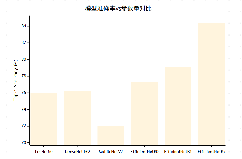
图4:不同模型准确率对比XY图表
5. 训练策略与优化
5.1 渐进式训练策略
EfficientNet的训练采用了渐进式策略,从小分辨率开始逐步增加:
python
class ProgressiveTraining:
    """EfficientNet渐进式训练策略"""
    def __init__(self, model, initial_size=128, target_size=224):
        self.model = model
        self.initial_size = initial_size
        self.target_size = target_size
        self.current_epoch = 0

    def get_current_resolution(self, epoch, total_epochs):
        """根据训练进度计算当前分辨率"""
        progress = epoch / total_epochs
        current_size = int(self.initial_size +
                          (self.target_size - self.initial_size) * progress)
        return current_size

    def create_data_loader(self, dataset, batch_size, resolution):
        """创建指定分辨率的数据加载器"""
        transform = transforms.Compose([
            transforms.Resize((resolution, resolution)),
            transforms.RandomHorizontalFlip(),
            transforms.ToTensor(),
            transforms.Normalize(mean=[0.485, 0.456, 0.406],
                               std=[0.229, 0.224, 0.225])
        ])

        dataset.transform = transform
        return DataLoader(dataset, batch_size=batch_size, shuffle=True)

# 训练配置
class EfficientNetTrainer:
    def __init__(self, model, device='cuda'):
        self.model = model.to(device)
        self.device = device
        self.optimizer = torch.optim.AdamW(
            model.parameters(),
            lr=0.016,  # 基础学习率
            weight_decay=1e-5
        )
        self.scheduler = torch.optim.lr_scheduler.CosineAnnealingLR(
            self.optimizer, T_max=350
        )
        self.criterion = nn.CrossEntropyLoss(label_smoothing=0.1)

    def train_epoch(self, dataloader, epoch):
        """训练一个epoch"""
        self.model.train()
        total_loss = 0
        correct = 0
        total = 0

        for batch_idx, (data, target) in enumerate(dataloader):
            data, target = data.to(self.device), target.to(self.device)

            # 前向传播
            self.optimizer.zero_grad()
            output = self.model(data)
            loss = self.criterion(output, target)

            # 反向传播
            loss.backward()
            self.optimizer.step()

            # 统计
            total_loss += loss.item()
            pred = output.argmax(dim=1, keepdim=True)
            correct += pred.eq(target.view_as(pred)).sum().item()
            total += target.size(0)

            if batch_idx % 100 == 0:
                print(f'Epoch: {epoch}, Batch: {batch_idx}, '
                      f'Loss: {loss.item():.4f}, '
                      f'Acc: {100.*correct/total:.2f}%')

        self.scheduler.step()
        return total_loss / len(dataloader), 100. * correct / total
5.2 数据增强策略
python
import torchvision.transforms as transforms
from PIL import Image
import random

class EfficientNetAugmentation:
    """EfficientNet专用数据增强"""
    def __init__(self, image_size=224):
        self.image_size = image_size

    def get_train_transform(self):
        """训练时的数据增强"""
        return transforms.Compose([
            transforms.RandomResizedCrop(self.image_size, scale=(0.08, 1.0)),
            transforms.RandomHorizontalFlip(p=0.5),
            transforms.ColorJitter(brightness=0.4, contrast=0.4,
                                 saturation=0.4, hue=0.1),
            transforms.ToTensor(),
            transforms.Normalize(mean=[0.485, 0.456, 0.406],
                               std=[0.229, 0.224, 0.225]),
            transforms.RandomErasing(p=0.25)  # 随机擦除
        ])

    def get_val_transform(self):
        """验证时的数据变换"""
        return transforms.Compose([
            transforms.Resize(int(self.image_size * 1.14)),  # 稍大一些
            transforms.CenterCrop(self.image_size),
            transforms.ToTensor(),
            transforms.Normalize(mean=[0.485, 0.456, 0.406],
                               std=[0.229, 0.224, 0.225])
        ])

# AutoAugment策略
class AutoAugment:
    """AutoAugment数据增强策略"""
    def __init__(self):
        self.policies = [
            # 策略1: 旋转 + 等化
            [('rotate', 0.9, 9), ('equalize', 0.8, 6)],
            # 策略2: 色彩 + 等化
            [('color', 0.4, 0), ('equalize', 0.6, 7)],
            # 更多策略...
        ]

    def __call__(self, img):
        policy = random.choice(self.policies)
        for operation, probability, magnitude in policy:
            if random.random() < probability:
                img = self.apply_operation(img, operation, magnitude)
        return img

    def apply_operation(self, img, operation, magnitude):
        """应用具体的增强操作"""
        if operation == 'rotate':
            angle = magnitude * 30 / 10  # 映射到角度
            return img.rotate(angle)
        elif operation == 'equalize':
            return transforms.functional.equalize(img)
        # 其他操作...
        return img
6. 实际应用案例
6.1 图像分类任务
python
class ImageClassifier:
    """基于EfficientNet的图像分类器"""
    def __init__(self, model_name='efficientnet-b0', num_classes=1000):
        self.model = self.load_pretrained_model(model_name, num_classes)
        self.transform = self.get_transform()

    def load_pretrained_model(self, model_name, num_classes):
        """加载预训练模型"""
        # 这里可以使用timm库或自定义实现
        model = create_efficientnet_b0()

        # 如果类别数不是1000,需要修改分类头
        if num_classes != 1000:
            model.head[-1] = nn.Linear(1280, num_classes)

        return model

    def get_transform(self):
        """获取预处理变换"""
        return transforms.Compose([
            transforms.Resize(256),
            transforms.CenterCrop(224),
            transforms.ToTensor(),
            transforms.Normalize(mean=[0.485, 0.456, 0.406],
                               std=[0.229, 0.224, 0.225])
        ])

    def predict(self, image_path):
        """预测单张图片"""
        # 加载图片
        image = Image.open(image_path).convert('RGB')

        # 预处理
        input_tensor = self.transform(image).unsqueeze(0)

        # 推理
        self.model.eval()
        with torch.no_grad():
            outputs = self.model(input_tensor)
            probabilities = F.softmax(outputs, dim=1)
            predicted_class = torch.argmax(probabilities, dim=1).item()
            confidence = probabilities[0][predicted_class].item()

        return predicted_class, confidence

    def batch_predict(self, image_paths, batch_size=32):
        """批量预测"""
        results = []

        for i in range(0, len(image_paths), batch_size):
            batch_paths = image_paths[i:i+batch_size]
            batch_tensors = []

            for path in batch_paths:
                image = Image.open(path).convert('RGB')
                tensor = self.transform(image)
                batch_tensors.append(tensor)

            # 批量推理
            batch_input = torch.stack(batch_tensors)
            self.model.eval()
            with torch.no_grad():
                outputs = self.model(batch_input)
                probabilities = F.softmax(outputs, dim=1)

            for j, prob in enumerate(probabilities):
                predicted_class = torch.argmax(prob).item()
                confidence = prob[predicted_class].item()
                results.append((batch_paths[j], predicted_class, confidence))

        return results

# 使用示例
classifier = ImageClassifier(num_classes=10)  # 假设10类分类任务
# predicted_class, confidence = classifier.predict('test_image.jpg')
# print(f"预测类别: {predicted_class}, 置信度: {confidence:.4f}")
6.2 迁移学习应用
EfficientNet 用户 预训练阶段 预训练阶段 EfficientNet ImageNet预训练 ImageNet预训练 EfficientNet 特征提取器 特征提取器 EfficientNet 权重固化 权重固化 微调阶段 微调阶段 用户 加载预训练权重 加载预训练权重 用户 替换分类头 替换分类头 用户 小学习率训练 小学习率训练 应用阶段 应用阶段 用户 特定任务推理 特定任务推理 用户 性能评估 性能评估 用户 部署上线 部署上线 EfficientNet迁移学习流程
图5:EfficientNet迁移学习用户旅程图
7. 模型优化与部署
7.1 模型量化
python
import torch.quantization as quantization

class EfficientNetQuantization:
    """EfficientNet模型量化"""
    def __init__(self, model):
        self.model = model

    def post_training_quantization(self, calibration_loader):
        """训练后量化"""
        # 设置量化配置
        self.model.eval()
        self.model.qconfig = quantization.get_default_qconfig('fbgemm')

        # 准备量化
        quantization.prepare(self.model, inplace=True)

        # 校准
        with torch.no_grad():
            for data, _ in calibration_loader:
                self.model(data)

        # 转换为量化模型
        quantized_model = quantization.convert(self.model, inplace=False)
        return quantized_model

    def quantization_aware_training(self, train_loader, epochs=10):
        """量化感知训练"""
        # 设置QAT配置
        self.model.train()
        self.model.qconfig = quantization.get_default_qat_qconfig('fbgemm')

        # 准备QAT
        quantization.prepare_qat(self.model, inplace=True)

        # 训练循环
        optimizer = torch.optim.Adam(self.model.parameters(), lr=1e-4)
        criterion = nn.CrossEntropyLoss()

        for epoch in range(epochs):
            for batch_idx, (data, target) in enumerate(train_loader):
                optimizer.zero_grad()
                output = self.model(data)
                loss = criterion(output, target)
                loss.backward()
                optimizer.step()

        # 转换为量化模型
        self.model.eval()
        quantized_model = quantization.convert(self.model, inplace=False)
        return quantized_model

# 模型压缩对比
def compare_model_sizes(original_model, quantized_model):
    """对比模型大小"""
    # 保存模型
    torch.save(original_model.state_dict(), 'original_model.pth')
    torch.save(quantized_model.state_dict(), 'quantized_model.pth')

    # 计算文件大小
    import os
    original_size = os.path.getsize('original_model.pth') / (1024 * 1024)  # MB
    quantized_size = os.path.getsize('quantized_model.pth') / (1024 * 1024)  # MB

    print(f"原始模型大小: {original_size:.2f} MB")
    print(f"量化模型大小: {quantized_size:.2f} MB")
    print(f"压缩比: {original_size/quantized_size:.2f}x")
7.2 模型部署优化
python
class EfficientNetDeployment:
    """EfficientNet部署优化"""
    def __init__(self, model):
        self.model = model

    def optimize_for_inference(self):
        """推理优化"""
        # 设置为评估模式
        self.model.eval()

        # 融合BN层
        self.fuse_bn_layers()

        # JIT编译
        self.model = torch.jit.script(self.model)

        return self.model

    def fuse_bn_layers(self):
        """融合BatchNorm层"""
        for module in self.model.modules():
            if isinstance(module, MBConvBlock):
                # 融合卷积和BN层
                torch.quantization.fuse_modules(
                    module,
                    [['expand_conv.0', 'expand_conv.1']],
                    inplace=True
                )

    def export_to_onnx(self, dummy_input, onnx_path):
        """导出ONNX格式"""
        torch.onnx.export(
            self.model,
            dummy_input,
            onnx_path,
            export_params=True,
            opset_version=11,
            do_constant_folding=True,
            input_names=['input'],
            output_names=['output'],
            dynamic_axes={
                'input': {0: 'batch_size'},
                'output': {0: 'batch_size'}
            }
        )
        print(f"模型已导出到: {onnx_path}")

    def benchmark_inference(self, input_size=(1, 3, 224, 224), num_runs=100):
        """推理性能基准测试"""
        import time

        dummy_input = torch.randn(input_size)

        # 预热
        for _ in range(10):
            with torch.no_grad():
                _ = self.model(dummy_input)

        # 计时
        start_time = time.time()
        for _ in range(num_runs):
            with torch.no_grad():
                _ = self.model(dummy_input)
        end_time = time.time()

        avg_time = (end_time - start_time) / num_runs * 1000  # ms
        fps = 1000 / avg_time

        print(f"平均推理时间: {avg_time:.2f} ms")
        print(f"推理FPS: {fps:.2f}")

        return avg_time, fps

# 部署示例
model = create_efficientnet_b0()
deployment = EfficientNetDeployment(model)

# 优化模型
optimized_model = deployment.optimize_for_inference()

# 性能测试
avg_time, fps = deployment.benchmark_inference()

# 导出ONNX
dummy_input = torch.randn(1, 3, 224, 224)
deployment.export_to_onnx(dummy_input, 'efficientnet_b0.onnx')
8. 未来发展趋势
8.1 EfficientNet演进路线
25% 20% 20% 15% 12% 8% EfficientNet技术发展重点分布 架构搜索优化 训练策略改进 模型压缩技术 多模态扩展 边缘计算适配 自监督学习
图6:EfficientNet技术发展重点分布饼图
"在深度学习的世界里,效率不是妥协,而是智慧的体现。EfficientNet告诉我们,最优的解决方案往往来自于对问题本质的深刻理解,而不是简单的资源堆砌。"
8.2 技术发展预测
EfficientNet的成功为我们指明了几个重要方向:
- 神经架构搜索的普及化:随着计算资源的增长,NAS技术将更加普及
- 复合缩放的广泛应用:这种设计思想将扩展到更多网络架构
- 效率优先的设计理念:在追求精度的同时,效率将成为重要考量
- 多模态模型的发展:EfficientNet的设计原则将应用于视觉-语言模型
总结
回顾这次EfficientNet的深度探索之旅,我深深被这个模型的设计哲学所震撼。它不仅仅是一个网络架构的改进,更是一种全新的思维方式------如何在有限的资源约束下达到最优的性能。
EfficientNet的复合缩放方法让我重新思考了网络设计的本质。传统的做法往往是单一维度的暴力扩展,而EfficientNet通过数学约束和系统性思考,找到了三个维度的最优平衡点。这种方法论的价值远超模型本身,它为我们提供了一个通用的框架来思考任何系统的优化问题。
在实际项目中,我发现EfficientNet的魅力不仅在于其优异的性能,更在于其出色的可扩展性。从B0到B7的系列化设计,让我们可以根据具体的应用场景和资源限制,选择最合适的模型变体。这种灵活性在工业应用中尤为重要,因为不同的部署环境往往有着截然不同的约束条件。
MBConv模块的设计也给我留下了深刻印象。它巧妙地融合了深度可分离卷积、Squeeze-and-Excitation注意力机制和残差连接,每一个组件都有其存在的理由,整体设计既优雅又高效。这种模块化的设计思想,让我们可以更好地理解和改进网络架构。
从训练策略的角度来看,EfficientNet采用的渐进式训练、AutoAugment数据增强等技术,展现了现代深度学习训练的精细化程度。这些技术的组合使用,不仅提升了模型的性能,也为我们提供了宝贵的经验和启发。
在模型部署方面,EfficientNet的量化友好性和推理效率,使其在边缘计算和移动设备上有着广阔的应用前景。随着5G和物联网的发展,这种高效的模型架构将发挥越来越重要的作用。
展望未来,我相信EfficientNet所代表的效率优先设计理念将继续影响深度学习的发展方向。在计算资源日益珍贵、环境保护意识不断增强的今天,如何用更少的资源做更多的事情,将成为技术发展的重要驱动力。
参考链接
- EfficientNet: Rethinking Model Scaling for Convolutional Neural Networks
- EfficientNetV2: Smaller Models and Faster Training
- MobileNets: Efficient Convolutional Neural Networks for Mobile Vision Applications
- Squeeze-and-Excitation Networks
- Neural Architecture Search with Reinforcement Learning
关键词标签
EfficientNet 复合缩放 MBConv 神经架构搜索 模型优化