MATLAB绘制9种最新的混沌系统
MATLAB代码:
Matlab
function chaos_gallery()
% ------------------------------------------------------------
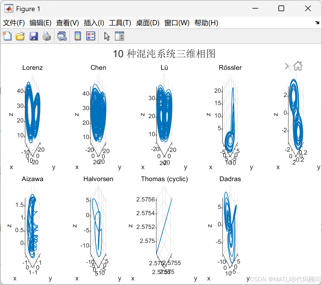
% 10 种代表性混沌系统相图(从经典到较新),统一绘制
% 系统列表:
% 1. Lorenz (σ=10, ρ=28, β=8/3)
% 2. Chen (a=35, b=3, c=28)
% 3. Lü (a=36, b=3, c=20)
% 4. Rössler (a=0.2, b=0.2, c=5.7)
% 5. Chua (α=9, β=14.286, m0=-1.143, m1=-0.714)
% 6. Aizawa (a=0.95, b=0.7, c=0.6, d=3.5, e=0.25, f=0.1)
% 7. Halvorsen (a=1.89)
% 8. Thomas (cyclic) (b=0.208186)
% 9. Dadras (a=3, b=2.7, c=1.7, d=2, e=9)
%
% 使用说明:
% - 直接运行 chaos_gallery 即可绘制 10 张 3D 相图
% - 如需更长积分或更细分辨率,修改 TSPAN 与 ODE 选项
% - 如只想画 2D 投影,见末尾可选代码段(已给模板)
% ------------------------------------------------------------
clc; close all; rng(1); % 固定随机种子,便于复现实验
% 全局积分设置
TSPAN = [0 80]; % 积分时间段(部分系统收敛较慢可适当加长)
odeopt = odeset('RelTol',1e-8,'AbsTol',1e-9,'MaxStep',0.05);
% 定义 10 个系统的配置:名称、方程、参数、初值
S = {};
% 1. Lorenz
S{end+1} = struct('name','Lorenz', ...
'f',@(t,x) lorenz_f(x,10,28,8/3), ...
'x0',[ -8; 7; 27 ]);
% 2. Chen
S{end+1} = struct('name','Chen', ...
'f',@(t,x) chen_f(x,35,3,28), ...
'x0',[ -10; 0; 37 ]);
% 3. Lü
S{end+1} = struct('name','Lü', ...
'f',@(t,x) lu_f(x,36,3,20), ...
'x0',[ -10; -5; 25 ]);
% 4. Rössler
S{end+1} = struct('name','Rössler', ...
'f',@(t,x) rossler_f(x,0.2,0.2,5.7), ...
'x0',[ 0; 1; 0 ]);
% 5. Chua
S{end+1} = struct('name','Chua', ...
'f',@(t,x) chua_f(x,9,14.286,-1.143,-0.714), ...
'x0',[ -0.1; 0; 0.1 ]);
% 6. Aizawa
S{end+1} = struct('name','Aizawa', ...
'f',@(t,x) aizawa_f(x,0.95,0.7,0.6,3.5,0.25,0.1), ...
'x0',[ 0.1; 0; 0 ]);
% 7. Halvorsen
S{end+1} = struct('name','Halvorsen', ...
'f',@(t,x) halvorsen_f(x,1.89), ...
'x0',[ 1; 0; 0 ]);
% 8. Thomas (cyclic)
S{end+1} = struct('name','Thomas (cyclic)', ...
'f',@(t,x) thomas_f(x,0.208186), ...
'x0',[ 1; 1; 1 ]);
% 9. Dadras
S{end+1} = struct('name','Dadras', ...
'f',@(t,x) dadras_f(x,3,2.7,1.7,2,9), ...
'x0',[ 2; 3; 1 ]);
% 绘图布局
tiledlayout(2,5,'Padding','compact','TileSpacing','compact');
% 主循环:积分 + 绘图
for k = 1:numel(S)
[t, X] = ode45(S{k}.f, TSPAN, S{k}.x0, odeopt);
% 去掉初期过渡(可选),增强吸引子形态
cut = max(1, round(0.1*length(t))); % 丢弃前 10% 时间点
Xp = X(cut:end,:);
nexttile;
plot3(Xp(:,1), Xp(:,2), Xp(:,3), 'LineWidth', 0.8);
grid on; axis tight; view(45,20);
title(S{k}.name, 'Interpreter','none');
xlabel('x'); ylabel('y'); zlabel('z');
end
sgtitle('9 种混沌系统三维相图');
% 是否保存图片
doSave = true;
if doSave
f = gcf;
f.Color = 'w';
print(f, 'chaos_gallery_3D.png', '-dpng', '-r300'); % 300 dpi
disp('已保存:chaos_gallery_3D.png');
end
% ===== 可选:绘制 2D 投影(例如 x--y 投影),开启下方代码块 =====
%{
figure('Color','w'); tiledlayout(2,5,'Padding','compact','TileSpacing','compact');
for k = 1:numel(S)
[t, X] = ode45(S{k}.f, TSPAN, S{k}.x0, odeopt);
cut = max(1, round(0.1*length(t)));
Xp = X(cut:end,:);
nexttile;
plot(Xp(:,1), Xp(:,2), 'LineWidth', 0.8);
axis equal tight; grid on;
title([S{k}.name ' (x--y)'], 'Interpreter','none');
xlabel('x'); ylabel('y');
end
sgtitle('10 种混沌系统二维投影(x--y)');
print(gcf, 'chaos_gallery_xy.png', '-dpng', '-r300');
%}
end
% ================== 各系统方程(子函数) ==================
function dx = lorenz_f(x,sigma,rho,beta)
% Lorenz 系统
dx = [ sigma*(x(2)-x(1));
x(1)*(rho - x(3)) - x(2);
x(1)*x(2) - beta*x(3) ];
end
function dx = chen_f(x,a,b,c)
% Chen 系统
dx = [ a*(x(2)-x(1));
(c-a)*x(1) - x(1)*x(3) + c*x(2);
x(1)*x(2) - b*x(3) ];
end
function dx = lu_f(x,a,b,c)
% Lü 系统
dx = [ a*(x(2)-x(1));
-x(1)*x(3) + c*x(2);
x(1)*x(2) - b*x(3) ];
end
function dx = rossler_f(x,a,b,c)
% Rössler 系统
dx = [ -x(2) - x(3);
x(1) + a*x(2);
b + x(3)*(x(1)-c) ];
end
function dx = chua_f(x,alpha,beta,m0,m1)
% Chua 电路
% 非线性电导 g(x) 为分段线性函数:
% g(x) = m1*x + 0.5*(m0-m1)*(|x+1|-|x-1|)
g = m1*x(1) + 0.5*(m0 - m1) * (abs(x(1)+1) - abs(x(1)-1));
dx = [ alpha*(x(2) - x(1) - g);
x(1) - x(2) + x(3);
-beta*x(2) ];
end
function dx = aizawa_f(x,a,b,c,d,e,f)
% Aizawa 系统
dx = [ (x(3)-b)*x(1) - d*x(2);
d*x(1) + (x(3)-b)*x(2);
c + a*x(3) - (x(3)^3)/3 - (x(1)^2 + x(2)^2)*(1 + e*x(3)) + f*x(3)*x(1)^3 ];
end
function dx = halvorsen_f(x,a)
% Halvorsen 系统
dx = [ -a*x(1) - 4*x(2) - 4*x(3) - x(2)^2;
-a*x(2) - 4*x(3) - 4*x(1) - x(3)^2;
-a*x(3) - 4*x(1) - 4*x(2) - x(1)^2 ];
end
function dx = thomas_f(x,b)
% Thomas(周期对称)系统
dx = [ sin(x(2)) - b*x(1);
sin(x(3)) - b*x(2);
sin(x(1)) - b*x(3) ];
end
function dx = dadras_f(x,a,b,c,d,e)
% Dadras 系统
dx = [ x(2) - a*x(1) + b*x(2)*x(3);
c*x(2) - x(1)*x(3) + x(3);
d*x(1)*x(2) - e*x(3) ];
end
function dx = rf_f(x,alpha,gamma)
% Rabinovich-Fabrikant 系统
dx = [ x(2)*(x(3)-1 + x(1)^2) + gamma*x(1);
x(1)*(3*x(3)+1 - x(1)^2) + gamma*x(2);
-2*x(3)*(alpha + x(1)*x(2)) ];
end