目录
- 一、链地址法
-
- [1.1 解决哈希冲突的思路](#1.1 解决哈希冲突的思路)
- [1.2 关于扩容](#1.2 关于扩容)
- [1.3 关于极端场景](#1.3 关于极端场景)
- 二、代码实现
-
- [2.1 节点结构框架](#2.1 节点结构框架)
- [2.2 insert 函数](#2.2 insert 函数)
-
- [2.2.1 插入逻辑](#2.2.1 插入逻辑)
- [2.2.2 扩容逻辑](#2.2.2 扩容逻辑)
- [2.2.3 插入函数测试](#2.2.3 插入函数测试)
- [2.3 find 和 erase 函数](#2.3 find 和 erase 函数)
- [2.4 质数表](#2.4 质数表)
- [2.5 析构函数](#2.5 析构函数)
- [2.5 解决 key 不能取模的问题](#2.5 解决 key 不能取模的问题)
-
- [测试 string 类型](#测试 string 类型)

前言
上期博客,我们讲解了哈希表的概念,并使用开放定址法实现了哈希表,本期博客我们将使用链地址法来实现哈希表。跳转上期博客:【C++】哈希表实现 - 开放定址法
一、链地址法
1.1 解决哈希冲突的思路
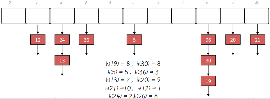
开放定址法 中所有的元素都放到哈希表里,链地址法 中所有的数据不再直接存储在哈希表中,哈希表中存储一个指针,没有数据映射这个位置时,这个指针为空,有多个数据映射到这个位置时,我们把这些冲突的数据链接成一个链表,挂在哈希表这个位置下面,链地址法也叫做哈希桶或者拉链法。
下面演示 {19,30,5,36,13,20,21,12,24,96} 等这一组值映射到M=11的表中。
1.2 关于扩容
开放定址法负载因子必须小于1,链地址法的负载因子就没有限制了,可以大于1。负载因子越大,哈希冲突的概率越高,空间利用率越高;负载因子越小,哈希冲突的概率越低,空间利用率越低;
stl中unordered系列最大负载因子基本控制在1,大于1就扩容,我们下面实现也使用这个方式。
1.3 关于极端场景
如果极端场景下,某个桶特别长怎么办?其实可以考虑使用全域散列法,这样就不容易被针对了。但是假设不是被针对了,用了全域散列法,但是偶然情况下,某个桶很长,查找效率很低怎么办?
这里在Java8的HashMap中当桶的长度超过一定阀值(8)时就把链表转换成红黑树。当然,一般情况下,不断扩容,单个桶很长的场景还是比较少的,C++没有考虑使用这种方式,还是使用的下面挂链表的方式。 我们在实现的时候也就直接挂链表了。
二、代码实现
2.1 节点结构框架
cpp
template<class K, class V>
struct HashNode
{
	// 单链表足以满足需求
	pair<K, V> _kv;
	HashNode<K, V>* _next;

	HashNode(const pair<K, V>& kv)
		:_kv(kv)
		,_next(nullptr)
	{ }
};

template<class K, class V>
class HashTable
{
public:
	typedef HashNode<K, V> Node;

	HashTable()
		:_tables(11)
		,_n(0)
	{ }
private:
	vector<Node*> _tables;
	size_t _n; // 实际存储的数据个数
};这里我们没有使用stl库中的list链表,而选择使用了原生链表,这样比较容易获取链表中的成员。
2.2 insert 函数
2.2.1 插入逻辑
cpp
bool insert(const pair<K, V>& kv)
{
	int hashi = kv.first % _tables.size();
	Node* newNode = new Node(kv);
	// 头插,尾插还要找尾
	// 第一个节点的地址在表里面
	newNode->_next = _tables[hashi];
	_tables[hashi] = newNode;
	++_n;

	return true;
}插入逻辑,我们选择头插,那就是将申请的新节点的_next指针指向旧的第一个节点,然后新节点成为新的第一个节点。不要忘了增加有效数据个数。
2.2.2 扩容逻辑
这里扩容时,就和前面的开放定址法不太一样,开放定址法是在insert函数中重新定义了一个类对象,这个类对象再调用insert函数,将数据重新定址,最后把类对象交换过来。但是放在链地址法这里,使用这样的方法会重新定义一遍节点,会造成空间的浪费,所以我们考虑把节点摘下来,重新挂。
cpp
bool insert(const pair<K, V>& kv)
{
// 负载因子 == 1,就扩容
if (_n == _tables.size())
{
vector<Node*> newtables(_tables.size() * 2);
for (int i = 0; i < _tables.size(); i++)
{
Node* cur = _tables[i];
while (cur)
{
// 存储 cur 的下一个节点
Node* next = cur->_next;
int hashi = cur->_kv.first % newtables.size();
cur->_next = newtables[hashi];
newtables[hashi] = cur;
cur = next; // 走到原链表的下一个节点
}
// 清空原链表节点数据
_tables[i] = nullptr;
}
// 交换新旧表
_tables.swap(newtables);
}
int hashi = kv.first % _tables.size();
Node* newNode = new Node(kv);
// 头插,尾插还要找尾
// 第一个节点的地址在表里面
newNode->_next = _tables[hashi];
_tables[hashi] = newNode;
++_n;
return true;
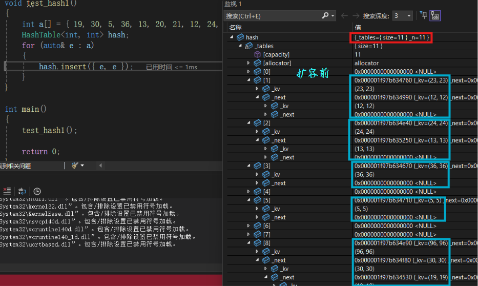
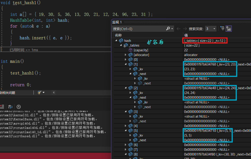
}2.2.3 插入函数测试
测试代码:
cpp
void test_hash1()
{
	int a[] = { 19, 30, 5, 36, 13, 20, 21, 12, 24, 96, 23, 31 };
	HashTable<int, int> hash;
	for (auto& e : a)
	{
		hash.insert({ e, e });
	}
}
测试结果 :
2.3 find 和 erase 函数
cpp
Node* find(const K& key)
{
	int hashi = key % _tables.size();
	Node* cur = _tables[hashi];
	while (cur)
	{
		// 找到返回节点地址
		if (cur->_kv.first == key)
		{
			return cur;
		}
		cur = cur->_next;
	}
	return nullptr;
}

bool erase(const K& key)
{
	int hashi = key % _tables.size();
	Node* cur = _tables[hashi];
	Node* pre = nullptr; // 保存 cur 的前一个节点
	while (cur)
	{
		// 找到返回节点地址
		if (cur->_kv.first == key)
		{
			// 要找的节点是表头
			if (pre == nullptr)
			{
				_tables[hashi] = cur->_next;
			}
			else
			{
				pre->_next = cur->_next;
			}
			delete cur;

			return true;
		}
		pre = cur;
		cur = cur->_next;
	}
测试代码
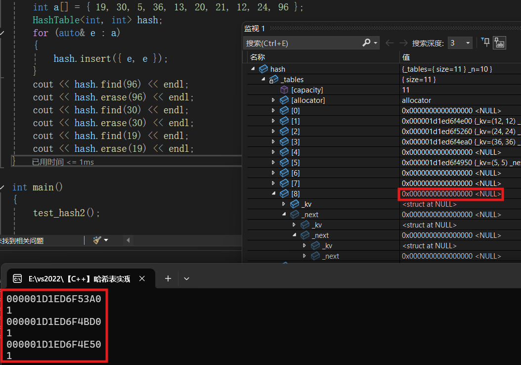
我们依旧按照之前的代码进行测试,我们发现96, 30, 19在一个桶中,我们把这三个全部删掉。
cpp
void test_hash2()
{
	int a[] = { 19, 30, 5, 36, 13, 20, 21, 12, 24, 96 };
	HashTable<int, int> hash;
	for (auto& e : a)
	{
		hash.insert({ e, e });
	}
	cout << hash.find(96) << endl;
	cout << hash.erase(96) << endl;
	cout << hash.find(30) << endl;
	cout << hash.erase(30) << endl;
	cout << hash.find(19) << endl;
	cout << hash.erase(19) << endl;
}
测试结果 :
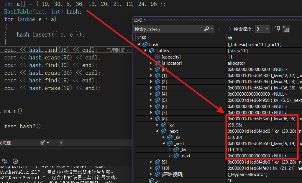
执行后 :
有了find之后,我们就可以再次完善insert了,完善不能插入相同元素的功能。
cpp
bool insert(const pair<K, V>& kv)
{
	if (find(kv.first))
	{
		return false;
	}
	// ...
}
2.4 质数表
和之前一样,我们这里的扩容更改为依旧使用stl源码里面给的近乎二倍增长的质数表。
cpp
template<class K, class V>
class HashTable
{
public:
	typedef HashNode<K, V> Node;

	HashTable()
		:_tables(__stl_next_prime(1)) // 开初始空间, 函数返回的是比 1 大且最接近 1 的值
		,_n(0)
	{ }

	inline unsigned long __stl_next_prime(unsigned long n)
	{
		// Note: assumes long is at least 32 bits.
		static const int __stl_num_primes = 28;
		static const unsigned long __stl_prime_list[__stl_num_primes] =
		{
			53, 97, 193, 389, 769,
			1543, 3079, 6151, 12289, 24593,
			49157, 98317, 196613, 393241, 786433,
			1572869, 3145739, 6291469, 12582917, 25165843,
			50331653, 100663319, 201326611, 402653189, 805306457,
			1610612741, 3221225473, 4294967291
		};
		const unsigned long* first = __stl_prime_list;
		const unsigned long* last = __stl_prime_list + __stl_num_primes;
		const unsigned long* pos = lower_bound(first, last, n);
		return pos == last ? *(last - 1) : *pos;
	}

	bool insert(const pair<K, V>& kv)
	{
		// 负载因子 == 1,就扩容
		if (_n == _tables.size())
		{
			vector<Node*> newtables(__stl_next_prime(_tables.size() + 1));

			// ...
		}

		// ...
	}
	// ...
private:
	vector<Node*> _tables;
	size_t _n; // 实际存储的数据个数
};测试代码:
cpp
void test_hash3()
{
	HashTable<int, int> hash;
	for (int i = 1; i < 200; i++)
	{
		hash.insert({ i, i });
		if (i == 100) // 可控断点
		{
			cout << endl;
		}
	}
}
测试结果 :
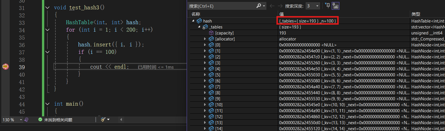
没有出现问题。
2.5 析构函数
cpp
~HashTable()
{
	for (int i = 0; i < _tables.size(); i++)
	{
		Node* cur = _tables[i];
		while (cur)
		{
			Node* next = cur->_next;
			delete cur;
			cur = next;
		}
		_tables[i] = nullptr;
	}
}
2.5 解决 key 不能取模的问题
这里的解决方法和我们的开放定址法相同,依旧使用仿函数把key转化成可以取模的整型值。
cpp
template<class K>
struct HashOfKey
{
	size_t operator()(const K& k)
	{
		return (size_t)k;
	}
};

template<>
struct HashOfKey<string>
{
	size_t operator()(const string& k)
	{
		size_t hs = 0;

		for (auto& e : k)
		{
			hs += e;
			hs *= 131; // 能够有效防止 "abcd" "bcda"的整型值一样的情况
		}
		return hs;
	}
};
cpp
template<class K, class V, class Hash = HashOfKey<K>>
class HashTable
{
public:
typedef HashNode<K, V> Node;
HashTable()
:_tables(__stl_next_prime(1)) // 开初始空间, 函数返回的是比 1 大且最接近 1 的值
,_n(0)
{ }
bool insert(const pair<K, V>& kv)
{
Hash kot;
// ...
// 负载因子 == 1,就扩容
if (_n == _tables.size())
{
vector<Node*> newtables(__stl_next_prime(_tables.size() + 1));
for (int i = 0; i < _tables.size(); i++)
{
Node* cur = _tables[i];
while (cur)
{
// 存储 cur 的下一个节点
Node* next = cur->_next;
int hashi = kot(cur->_kv.first) % newtables.size();
// ...
}
// ...
}
int hashi = kot(kv.first) % _tables.size();
// ...
return true;
}
Node* find(const K& key)
{
Hash kot;
size_t hashi = kot(key) % _tables.size();
// ...
while (cur)
{
// 找到返回节点地址
if (kot(cur->_kv.first) == kot(key))
// ...
}
return nullptr;
}
bool erase(const K& key)
{
Hash kot;
size_t hashi = kot(key) % _tables.size();
// ...
while (cur)
{
// 找到返回节点地址
if (kot(cur->_kv.first) == kot(key))
{
// ...
}
// ...
}
return false;
}
private:
vector<Node*> _tables;
size_t _n; // 实际存储的数据个数
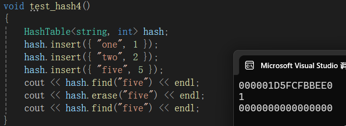
};测试 string 类型
测试代码:
cpp
void test_hash4()
{
	HashTable<string, int> hash;
	hash.insert({ "one", 1 });
	hash.insert({ "two", 2 });
	hash.insert({ "five", 5 });
	cout << hash.find("five") << endl;
	cout << hash.erase("five") << endl;
	cout << hash.find("five") << endl;
}测试结果:
总结:
以上就是本期博客分享的全部内容啦!如果觉得文章还不错的话可以三连支持一下,你的支持就是我前进最大的动力!
技术的探索永无止境! 道阻且长,行则将至!后续我会给大家带来更多优质博客内容,欢迎关注我的CSDN账号,我们一同成长!
(~ ̄▽ ̄)~