脚本优化--visium的细胞niche与共定位(R版本)

作者，Evil Genius

今天我们拉群，2025番外--linux、R、python培训https://mp.weixin.qq.com/s/8E1vYJMNhe5m0DXieBHfzA?payreadticket=HM3XzM3dAiSdVyi83oiJ3UWd-zPIOKO1EMMnYwy9ASu_scWj_WEje8Xwiwq_z8JvgcLDfd0&scene=1&click_id=1, 这是所有将来从事生物信息行业的第一课，也是现在入职诺禾、华大等上市公司的必备技能。

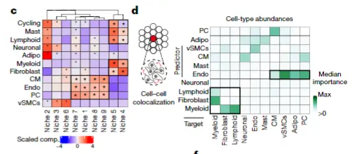
今天更新脚本，visium的细胞niche与共定位

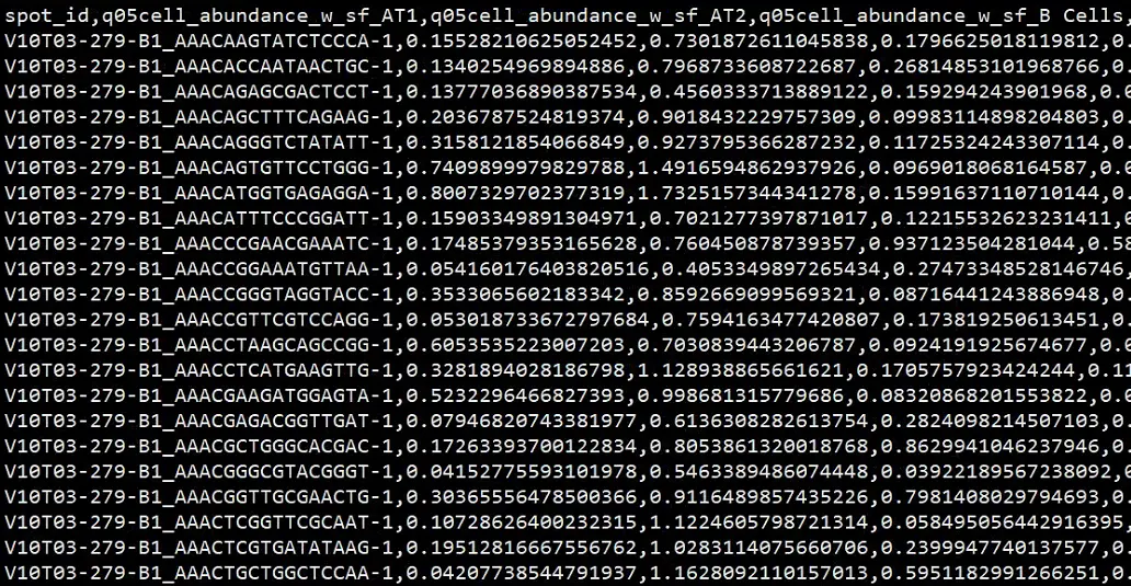
单细胞空间联合推荐cell2location, 拿到联合后的结果，注意联合的时候尽量样本要匹配，联合关键的参数在课堂上都已经有详细的讲解。

我们来更新脚本

library(compositions)
library(tidyverse)
library(clustree)
library(uwot)
library(scran)
library(cluster)

integrated_compositions = read.csv('cell2location的联合矩阵')

关键的一步，矩阵转换, 这个转换是等距对数比变换 (Isometric Log-Ratio Transformation)，是处理比例、百分比等相对组成数据的专业方法。

其中ilr转换核心作用是解决成分数据的闭合性约束问题，使其能够在标准的多元统计方法中使用。

成分数据的根本问题

成分数据具有"闭合性"（总和为常数，如100%），这导致：

1、成分数据具有"闭合性"（总和为常数，如100%）：伪相关性问题

2、非欧几里得几何：成分空间是单形空间，不是欧几里得空间，不能直接应用常规统计方法。

ilr转换的核心作用

1、消除闭合约束

2、保持等距性质

3. 实现坐标系统转换

# Generate ILR transformation
baseILR <- ilrBase(x = integrated_compositions,method = "basic")

cell_ilr <- as.matrix(ilr(integrated_compositions, baseILR))
colnames(cell_ilr) <- paste0("ILR_", 1:ncol(cell_ilr))

# Make community graph
k_vect <- c(10, 20,30)
k_vect <- set_names(k_vect, paste0("k_",k_vect))

cluster_info <- map(k_vect, function(k) {
  print(k)
  print("Generating SNN")
  snn_graph <- scran::buildSNNGraph(x = t(cell_ilr %>% as.data.frame() %>% as.matrix()), k = k)
  print("Louvain clustering")
  clust.louvain <- igraph::cluster_louvain(snn_graph)
  clusters <- tibble(cluster = clust.louvain$membership,
                     spot_id = rownames(cell_ilr))
})

cluster_info <- cluster_info %>% 
  enframe() %>%
  unnest() %>%
  pivot_wider(names_from = name,
              values_from = cluster)

k_vect <- set_names(names(k_vect))

subsampling_mean_ss <- map(k_vect, function(k) {
  print(k)
  
  cluster_info_summary <- cluster_info %>%
    group_by_at(k) %>%
    summarize(ncells = floor(n() * 0.3))
  
  cells <- cluster_info %>%
    dplyr::select_at(c("spot_id", k)) %>%
    group_by_at(k) %>%
    nest() %>%
    left_join(cluster_info_summary) %>%
    mutate(data = map(data, ~ .x[[1]])) %>%
    mutate(selected_cells = map2(data, ncells, function(dat,n) {
      sample(dat, n)
    })) %>%
    pull(selected_cells) %>%
    unlist()
  
  dist_mat <- dist(cell_ilr[cells, ])
  
  k_vect <- purrr::set_names(cluster_info[[k]], cluster_info[["spot_id"]])[cells]
  
  sil <- cluster::silhouette(x = k_vect, dist = dist_mat)
  
  mean(sil[, 'sil_width'])
  
})

subsampling_mean_ss <- enframe(subsampling_mean_ss) %>% 
  unnest() %>%
  dplyr::filter()

niche_resolution <- dplyr::filter(subsampling_mean_ss, 
                       value == max(value)) %>%
  pull(name)

plt <- comp_umap %>%
  ggplot(aes(x = V1, y = V2, 
             color = as.character(k_50))) +
  ggrastr::geom_point_rast(size = 0.1) +
  theme_classic() +
  xlab("UMAP1") +
  ylab("UMAP2") +
  guides(colour = guide_legend(override.aes = list(size=4)))

plot(plt)

cts <- set_names(colnames(integrated_compositions))

walk(cts, function(ct){
  
  plot_df <- comp_umap %>%
    mutate(ct_prop = log_comps[ , ct])
  
  plt <- plot_df %>%
    ggplot(aes(x = V1, y = V2, 
               color = ct_prop)) +
    ggrastr::geom_point_rast(size = 0.07) +
    theme_classic() +
    ggtitle(ct) +
    xlab("UMAP1") +
    ylab("UMAP2")
  
  plot(plt)
  
})

dev.off()

# Make the niche annotation meta-data

cluster_info <- comp_umap %>%
  dplyr::select(c("row_id","k_50")) %>%
  dplyr::rename("niche" = k_50) %>%
  dplyr::mutate(ct_niche = paste0("niche_", niche))

niche_summary_pat <- integrated_compositions %>%
  as.data.frame() %>%
  rownames_to_column("row_id") %>%
  pivot_longer(-row_id,values_to = "ct_prop", 
               names_to = "cell_type") %>%
  left_join(cluster_info) %>%
  mutate(orig.ident = strsplit(row_id, "[..]") %>%
           map_chr(., ~ .x[1])) %>%
  group_by(orig.ident, ct_niche, cell_type) %>%
  summarize(median_ct_prop = median(ct_prop))
  
niche_summary <- niche_summary_pat %>%
  ungroup() %>%
  group_by(ct_niche, cell_type) %>%
  summarise(patient_median_ct_prop = median(median_ct_prop))

# Data manipulation to have clustered data

niche_summary_mat <- niche_summary %>%
  pivot_wider(values_from = patient_median_ct_prop, 
              names_from =  cell_type, values_fill = 0) %>%
  column_to_rownames("ct_niche") %>%
  as.matrix()

niche_order <- hclust(dist(niche_summary_mat))
niche_order <- niche_order$labels[niche_order$order]

ct_order <- hclust(dist(t(niche_summary_mat)))
ct_order <- ct_order$labels[ct_order$order]

# Find characteristic cell types of each niche
# We have per patient the proportion of each cell-type in each niche

run_wilcox_up <- function(prop_data) {
  
  prop_data_group <- prop_data[["ct_niche"]] %>%
    unique() %>%
    set_names()
  
  map(prop_data_group, function(g) {
    
    test_data <- prop_data %>%
      mutate(test_group = ifelse(ct_niche == g,
                                 "target", "rest")) %>%
      mutate(test_group = factor(test_group,
                                 levels = c("target", "rest")))
    
    wilcox.test(median_ct_prop ~ test_group, 
                data = test_data,
                alternative = "greater") %>%
      broom::tidy()
  }) %>% enframe("ct_niche") %>%
    unnest()
  
}

wilcoxon_res <- niche_summary_pat %>%
  ungroup() %>%
  group_by(cell_type) %>%
  nest() %>%
  mutate(wres = map(data, run_wilcox_up)) %>%
  dplyr::select(wres) %>%
  unnest() %>%
  ungroup() %>%
  mutate(p_corr = p.adjust(p.value))

wilcoxon_res <- wilcoxon_res %>%
  mutate(significant = ifelse(p_corr <= 0.15, "*", ""))

write.table(niche_summary_pat, file = "./results/niche_mapping/ct_niches/niche_summary_pat.txt", 
            col.names = T, row.names = F, quote = F, sep = "\t")

write.table(wilcoxon_res, file = "./results/niche_mapping/ct_niches/wilcoxon_res_cells_niches.txt", 
            col.names = T, row.names = F, quote = F, sep = "\t")

mean_ct_prop_plt <- niche_summary %>%
  left_join(wilcoxon_res, by = c("ct_niche", "cell_type")) %>%
  mutate(cell_type = factor(cell_type, levels = ct_order),
         ct_niche = factor(ct_niche, levels = niche_order)) %>%
  ungroup() %>%
  group_by(cell_type) %>%
  mutate(scaled_pat_median = (patient_median_ct_prop - mean(patient_median_ct_prop))/sd(patient_median_ct_prop)) %>%
  ungroup() %>%
  ggplot(aes(x = cell_type, y = ct_niche, fill = scaled_pat_median)) +
  geom_tile() +
  geom_text(aes(label = significant)) +
  theme(axis.text.x = element_text(angle = 90, hjust = 1, vjust = 0.5, size = 12),
        legend.position = "bottom",
        plot.margin = unit(c(0, 0, 0, 0), "cm"),
        axis.text.y = element_text(size=12)) +
  scale_fill_gradient(high = "#ffd89b", low = "#19547b")
  

# Finally describe the proportions of those niches in all the data
cluster_counts <- cluster_info %>%
  dplyr::select_at(c("row_id", "ct_niche")) %>%
  group_by(ct_niche) %>%
  summarise(nspots = length(ct_niche)) %>%
  mutate(prop_spots = nspots/sum(nspots))

write_csv(cluster_counts, file = "./results/niche_mapping/ct_niches/niche_prop_summary.csv")

barplts <- cluster_counts %>%
  mutate(ct_niche = factor(ct_niche, levels = niche_order)) %>%
  ggplot(aes(y = ct_niche, x = prop_spots)) +
  geom_bar(stat = "identity") +
  theme_classic() + ylab("") +
  theme(axis.text.y = element_blank(),
        plot.margin = unit(c(0, 0, 0, 0), "cm"),
        axis.text.x = element_text(size=12)) 

niche_summary_plt <- cowplot::plot_grid(mean_ct_prop_plt, barplts, align = "hv", axis = "tb")

pdf("./results/niche_mapping/ct_niches/characteristic_ct_niches.pdf", height = 3, width = 6)

plot(niche_summary_plt)

dev.off()

pdf(file = "./results/niche_mapping/ct_niches/niche_summary_pat.pdf", height = 5, width = 8)
niche_summary_pat %>%
  ggplot(aes(x = ct_niche, y  = median_ct_prop)) +
  geom_boxplot() +
  theme(axis.text.x = element_text(angle = 90, hjust = 1, vjust = 0.5)) +
  facet_wrap(.~cell_type, ncol = 3,scales = "free_y")
dev.off()

生活很好，有你更好