基于深度卷积神经网络与迁移学习的动物图像分类

🐈基于深度卷积神经网络与迁移学习的动物图像分类

---

代码数据集来源

🔬项目概述

动物图像分类是一项复杂任务，通过人工智能算法根据视觉特征识别和归类动物。这项技术具有广泛应用场景，包括野生动物保护、兽医学乃至农业领域。随着深度学习与计算机视觉技术的发展，如今已能构建高精度、高效率的动物图像分类系统，实现海量图像的实时分析。

动物图像分类的主要挑战在于处理海量视觉数据。这些数据形态多样，既包含低画质的红外相机影像，也涵盖专业摄影师拍摄的高清图片。此外，动物的外观会因年龄、性别、地域等因素产生显著差异。为应对这些挑战，研究者通常采用能从大型数据集学习并具备良好泛化能力的深度学习模型。

技术伦理是动物图像分类的另一重要维度。虽然AI驱动的野生动物监测系统有望革新保护工作，但也引发了关于隐私保护、数据安全与动物福利的担忧。研究人员和开发者必须优先考虑伦理规范，与保护主义者、动物权益组织及原住民社区等利益相关方协作，确保相关技术得到负责任的应用并创造普惠价值。

❗作者说明：

请确保使用GPU加速器从上至下顺序运行所有单元。部分单元格包含Linux命令，这一点需要特别注意。欢迎提出任何改进建议与意见，我们将不胜感激。编码愉快！

---

🏗️导入必要的库

# 导入数据科学库
import numpy as np
import pandas as pd
import tensorflow as tf
from sklearn.model_selection import train_test_split
import itertools
import random

# 导入可视化库
import matplotlib.pyplot as plt
import matplotlib.cm as cm
import cv2
import seaborn as sns

# Tensorflow 库
from tensorflow import keras
from tensorflow.keras import layers,models
from tensorflow.keras.preprocessing.image import ImageDataGenerator
from tensorflow.keras.layers import Dense, Dropout, BatchNormalization
from tensorflow.keras.callbacks import Callback, EarlyStopping,ModelCheckpoint, ReduceLROnPlateau
from tensorflow.keras import Model
from tensorflow.keras.layers.experimental import preprocessing
from tensorflow.keras.optimizers import Adam

# 系统库
from pathlib import Path
import os.path

# 评估指标
from sklearn.metrics import classification_report, confusion_matrix

sns.set_style('darkgrid')  # 设置 seaborn 绘图风格为暗网格

# 设定所有随机种子以便复现结果
def seed_everything(seed=42):
    # 设置TensorFlow的随机种子
    tf.random.set_seed(seed)
    
    # 设置NumPy的随机种子
    np.random.seed(seed)
    
    # 设置Python随机库的种子
    random.seed(seed)
    
    # 强制TensorFlow使用单线程
    # 多线程可能导致结果不可复现
    session_conf = tf.compat.v1.ConfigProto(
        intra_op_parallelism_threads=1,    # 设置操作内并行线程数为1
        inter_op_parallelism_threads=1     # 设置操作间并行线程数为1
    )

    # 确保TensorFlow在可能的情况下使用确定性操作
    tf.compat.v1.set_random_seed(seed)

    # 创建会话并设置会话配置
    sess = tf.compat.v1.Session(graph=tf.compat.v1.get_default_graph(), config=session_conf)
    tf.compat.v1.keras.backend.set_session(sess)

# 执行种子设置函数
seed_everything()

🤙创建辅助函数

# 下载辅助函数文件
!wget https://raw.githubusercontent.com/mrdbourke/tensorflow-deep-learning/main/extras/helper_functions.py

# 导入用于我们笔记本文档的一系列辅助函数
from helper_functions import create_tensorboard_callback, plot_loss_curves, unzip_data, compare_historys, walk_through_dir, pred_and_plot

输出:

--2023-04-08 09:57:27--  https://raw.githubusercontent.com/mrdbourke/tensorflow-deep-learning/main/extras/helper_functions.py
Resolving raw.githubusercontent.com (raw.githubusercontent.com)... 185.199.108.133, 185.199.109.133, 185.199.110.133, ...
Connecting to raw.githubusercontent.com (raw.githubusercontent.com)|185.199.108.133|:443... connected.
HTTP request sent, awaiting response... 200 OK
Length: 10246 (10K) [text/plain]
Saving to: 'helper_functions.py'

helper_functions.py 100%[===================>]  10.01K  --.-KB/s    in 0s      

2023-04-08 09:57:27 (51.9 MB/s) - 'helper_functions.py' saved [10246/10246]

6/10246]

📥加载和转换数据

BATCH_SIZE = 32
TARGET_SIZE = (224, 224)

# 遍历每个目录
dataset = "/animals10/raw-img"
walk_through_dir(dataset)

输出:

There are 10 directories and 0 images in '/kaggle/input/animals10/raw-img'.
There are 0 directories and 2623 images in '/kaggle/input/animals10/raw-img/cavallo'.
There are 0 directories and 1820 images in '/kaggle/input/animals10/raw-img/pecora'.
There are 0 directories and 1446 images in '/kaggle/input/animals10/raw-img/elefante'.
There are 0 directories and 1668 images in '/kaggle/input/animals10/raw-img/gatto'.
There are 0 directories and 1862 images in '/kaggle/input/animals10/raw-img/scoiattolo'.
There are 0 directories and 3098 images in '/kaggle/input/animals10/raw-img/gallina'.
There are 0 directories and 4821 images in '/kaggle/input/animals10/raw-img/ragno'.
There are 0 directories and 1866 images in '/kaggle/input/animals10/raw-img/mucca'.
There are 0 directories and 4863 images in '/kaggle/input/animals10/raw-img/cane'.
There are 0 directories and 2112 images in '/kaggle/input/animals10/raw-img/farfalla'.

📅 将数据整理到数据框中

第一列 filepaths 包含每个图像的文件路径位置。第二列 labels 则包含来自文件路径的对应图像的类别标签

def convert_path_to_df(dataset):
    image_dir = Path(dataset)

    # 获取文件路径和标签
    filepaths = list(image_dir.glob(r'**/*.JPG')) + list(image_dir.glob(r'**/*.jpg')) + list(image_dir.glob(r'**/*.jpeg')) + list(image_dir.glob(r'**/*.PNG'))

    labels = list(map(lambda x: os.path.split(os.path.split(x)[0])[1], filepaths))

    filepaths = pd.Series(filepaths, name='Filepath').astype(str)
    labels = pd.Series(labels, name='Label')

    # 合并文件路径和标签
    image_df = pd.concat([filepaths, labels], axis=1)
    return image_df

image_df = convert_path_to_df(dataset)

# 检查数据集中的损坏图像
import PIL
from pathlib import Path
from PIL import UnidentifiedImageError

path = Path(dataset).rglob("*.jpg")
for img_p in path:
    try:
        img = PIL.Image.open(img_p)
    except PIL.UnidentifiedImageError:
            print(img_p)

# 获取每个标签的数值计数
label_counts = image_df['Label'].value_counts()

# 创建图形和坐标轴
fig, axes = plt.subplots(nrows=1, ncols=1, figsize=(20, 6))

# 绘制条形图
sns.barplot(x=label_counts.index, y=label_counts.values, alpha=0.8, palette='pastel', ax=axes)
axes.set_title('Distribution of Labels in Image Dataset', fontsize=16)
axes.set_xlabel('Label', fontsize=14)
axes.set_ylabel('Count', fontsize=14)
axes.set_xticklabels(label_counts.index, rotation=45)

# 添加总标题到图形
fig.suptitle('Image Dataset Label Distribution', fontsize=20)

# 调整绘图和标题之间的间距
fig.subplots_adjust(top=0.85)

# 显示图形
plt.show()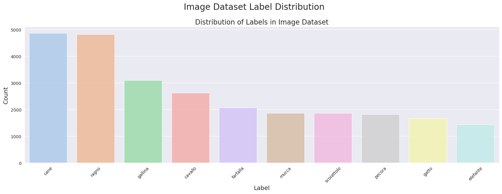

🔭可视化数据集中的图像

# 显示数据集的16张图片及其标签
random_index = np.random.randint(0, len(image_df), 16)
fig, axes = plt.subplots(nrows=4, ncols=4, figsize=(10, 10),
                        subplot_kw={'xticks': [], 'yticks': []})

for i, ax in enumerate(axes.flat):
    ax.imshow(plt.imread(image_df.Filepath[random_index[i]]))
    ax.set_title(image_df.Label[random_index[i]])
plt.tight_layout()
plt.show()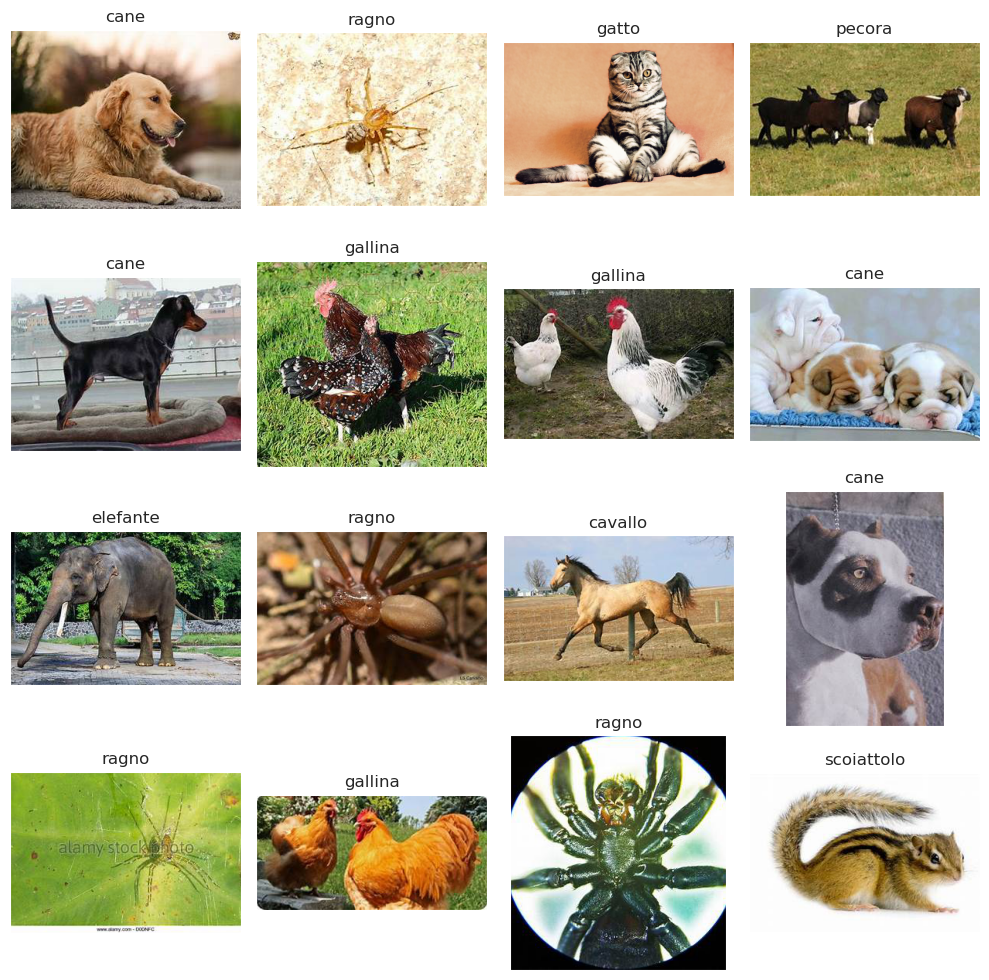

🧮计算错误级别分析

下面的代码用于在动物图像分类任务中对图像进行错误级别分析（ELA）。

compute_ela_cv() 函数接受图像路径和质量参数，使用给定质量的JPEG压缩对图像进行压缩，并计算压缩图像与原始图像之间的绝对差异。该差异乘以一个比例因子并作为ELA图像返回。

convert_to_ela_image() 函数接受图像路径和质量参数，使用给定质量的JPEG压缩对图像进行压缩，计算压缩图像与原始图像之间的绝对差异，并返回ELA图像。ELA图像使用原始图像和压缩图像之间的像素值差异计算，并进行归一化以增强差异。

random_sample() 函数接受目录路径和可选的文件扩展名，并从该目录返回具有指定扩展名（如果提供）的随机文件路径。

最后，代码使用 compute_ela_cv() 函数为从动物图像测试数据集中随机选择的图像生成一组ELA图像。ELA图像以递减的质量级别生成，导致压缩级别增加，从而错误级别也随之增加。使用 matplotlib 绘制生成的图像。

总体而言，这段代码提供了一种可视化分析不同JPEG压缩级别对动物图像影响的方法，可用于在动物图像分类任务中确定图像压缩的最佳质量级别。

def compute_ela_cv(path, quality):
    temp_filename = 'temp_file_name.jpeg'
    SCALE = 15
    orig_img = cv2.imread(path)
    orig_img = cv2.cvtColor(orig_img, cv2.COLOR_BGR2RGB)
    
    cv2.imwrite(temp_filename, orig_img, [cv2.IMWRITE_JPEG_QUALITY, quality])

    # 读取压缩后的图像
    compressed_img = cv2.imread(temp_filename)

    # 计算原始图像和压缩图像之间的绝对差异并乘以比例因子
    diff = SCALE * cv2.absdiff(orig_img, compressed_img)
    return diff


def convert_to_ela_image(path, quality):
    temp_filename = 'temp_file_name.jpeg'
    ela_filename = 'temp_ela.png'
    image = Image.open(path).convert('RGB')
    image.save(temp_filename, 'JPEG', quality = quality)
    temp_image = Image.open(temp_filename)

    ela_image = ImageChops.difference(image, temp_image)

    extrema = ela_image.getextrema()
    max_diff = max([ex[1] for ex in extrema])
    if max_diff == 0:
        max_diff = 1

    scale = 255.0 / max_diff
    ela_image = ImageEnhance.Brightness(ela_image).enhance(scale)
    
    return ela_image


def random_sample(path, extension=None):
    if extension:
        items = Path(path).glob(f'*.{extension}')
    else:
        items = Path(path).glob(f'*')
        
    items = list(items)
        
    p = random.choice(items)
    return p.as_posix()

# 查看数据集中的随机样本
p = random_sample('/animals10/raw-img/cane')
orig = cv2.imread(p)
orig = cv2.cvtColor(orig, cv2.COLOR_BGR2RGB) / 255.0
init_val = 100
columns = 3
rows = 3

fig=plt.figure(figsize=(15, 10))
for i in range(1, columns*rows +1):
    quality=init_val - (i-1) * 8
    img = compute_ela_cv(path=p, quality=quality)
    if i == 1:
        img = orig.copy()
    ax = fig.add_subplot(rows, columns, i) 
    ax.title.set_text(f'质量: {quality}')
    plt.imshow(img)
plt.show()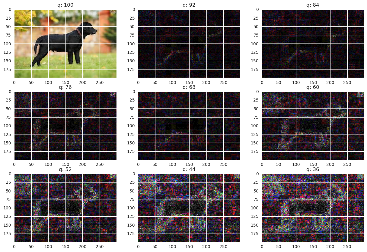

📝数据预处理

数据将被分为三个不同的类别：训练集、验证集和测试集。训练数据将用于训练深度学习CNN模型，其参数将通过验证数据进行微调。最后，将使用测试数据（模型之前未见过的数据）评估数据的性能。

# 分离训练集和测试集数据
train_df, test_df = train_test_split(image_df, test_size=0.2, shuffle=True, random_state=42)

train_generator = ImageDataGenerator(
    preprocessing_function=tf.keras.applications.efficientnet.preprocess_input,
    validation_split=0.2
)

test_generator = ImageDataGenerator(
    preprocessing_function=tf.keras.applications.efficientnet.preprocess_input,
)

# 将数据分为三个类别：训练集、验证集和测试集
train_images = train_generator.flow_from_dataframe(
    dataframe=train_df,
    x_col='Filepath',
    y_col='Label',
    target_size=TARGET_SIZE,
    color_mode='rgb',
    class_mode='categorical',
    batch_size=BATCH_SIZE,
    shuffle=True,
    seed=42,
    subset='training'
)

val_images = train_generator.flow_from_dataframe(
    dataframe=train_df,
    x_col='Filepath',
    y_col='Label',
    target_size=TARGET_SIZE,
    color_mode='rgb',
    class_mode='categorical',
    batch_size=BATCH_SIZE,
    shuffle=True,
    seed=42,
    subset='validation'
)

test_images = test_generator.flow_from_dataframe(
    dataframe=test_df,
    x_col='Filepath',
    y_col='Label',
    target_size=TARGET_SIZE,
    color_mode='rgb',
    class_mode='categorical',
    batch_size=BATCH_SIZE,
    shuffle=False
)

输出:

Found 16722 validated image filenames belonging to 10 classes.
Found 4180 validated image filenames belonging to 10 classes.
Found 5226 validated image filenames belonging to 10 classes.

# 数据增强步骤
augment = tf.keras.Sequential([
  layers.experimental.preprocessing.Resizing(224,224),
  layers.experimental.preprocessing.Rescaling(1./255),
  layers.experimental.preprocessing.RandomFlip("horizontal"),
  layers.experimental.preprocessing.RandomRotation(0.1),
  layers.experimental.preprocessing.RandomZoom(0.1),
  layers.experimental.preprocessing.RandomContrast(0.1),
])

🤹训练模型

模型图像将使用名为EfficientNetB7的预训练CNN模型进行处理。将使用三个回调函数来监控训练过程，分别是：模型检查点、早停法和TensorBoard回调。模型超参数摘要如下所示：

批大小 : 32
训练轮数 : 100
输入形状 : (224, 224, 3)
输出层: 10

# 加载预训练模型
pretrained_model = tf.keras.applications.efficientnet.EfficientNetB7(
    input_shape=(224, 224, 3),
    include_top=False,
    weights='imagenet',
    pooling='max'
)

pretrained_model.trainable = False

输出:

Downloading data from https://storage.googleapis.com/keras-applications/efficientnetb7_notop.h5
258076736/258076736 [==============================] - 8s 0us/step

# 创建检查点回调
checkpoint_path = "animals_classification_model_checkpoint"
checkpoint_callback = ModelCheckpoint(checkpoint_path,
                                      save_weights_only=True,
                                      monitor="val_accuracy",
                                      save_best_only=True)

# 设置早停回调，如果模型的验证损失在5个周期内没有改善则停止训练
early_stopping = EarlyStopping(monitor="val_loss", # 监控验证损失指标
                               patience=5,
                               restore_best_weights=True) # 如果验证损失连续5个周期没有改善，停止训练

# 设置学习率衰减回调
reduce_lr = ReduceLROnPlateau(monitor='val_loss', factor=0.2, patience=3, min_lr=1e-6)

🚄训练模型

inputs = pretrained_model.input
x = augment(inputs)

x = Dense(128, activation='relu')(pretrained_model.output)
x = BatchNormalization()(x)
x = Dropout(0.45)(x)
x = Dense(256, activation='relu')(x)
x = BatchNormalization()(x)
x = Dropout(0.45)(x)


outputs = Dense(10, activation='softmax')(x)

model = Model(inputs=inputs, outputs=outputs)

model.compile(
    optimizer=Adam(0.00001),
    loss='categorical_crossentropy',
    metrics=['accuracy']
)

history = model.fit(
    train_images,
    steps_per_epoch=len(train_images),
    validation_data=val_images,
    validation_steps=len(val_images),
    epochs=100,
    callbacks=[
        early_stopping,
        create_tensorboard_callback("training_logs", 
                                    "animals_classification"),
        checkpoint_callback,
        reduce_lr
    ]
)

输出:

Saving TensorBoard log files to: training_logs/animals_classification/20230408-095840
Epoch 1/100

输出:

2023-04-08 09:58:59.795552: E tensorflow/core/grappler/optimizers/meta_optimizer.cc:954] layout failed: INVALID_ARGUMENT: Size of values 0 does not match size of permutation 4 @ fanin shape inmodel/block1b_drop/dropout/SelectV2-2-TransposeNHWCToNCHW-LayoutOptimizer

输出:

523/523 [==============================] - 202s 335ms/step - loss: 2.5555 - accuracy: 0.2662 - val_loss: 1.1115 - val_accuracy: 0.6761 - lr: 1.0000e-05
Epoch 2/100
523/523 [==============================] - 150s 286ms/step - loss: 1.5455 - accuracy: 0.5141 - val_loss: 0.6618 - val_accuracy: 0.8407 - lr: 1.0000e-05
Epoch 3/100
523/523 [==============================] - 150s 286ms/step - loss: 1.0930 - accuracy: 0.6566 - val_loss: 0.4573 - val_accuracy: 0.8945 - lr: 1.0000e-05
Epoch 4/100
523/523 [==============================] - 150s 286ms/step - loss: 0.8465 - accuracy: 0.7360 - val_loss: 0.3439 - val_accuracy: 0.9208 - lr: 1.0000e-05
Epoch 5/100
523/523 [==============================] - 150s 287ms/step - loss: 0.6832 - accuracy: 0.7938 - val_loss: 0.2753 - val_accuracy: 0.9371 - lr: 1.0000e-05
Epoch 6/100
523/523 [==============================] - 150s 287ms/step - loss: 0.5716 - accuracy: 0.8305 - val_loss: 0.2334 - val_accuracy: 0.9447 - lr: 1.0000e-05
Epoch 7/100
523/523 [==============================] - 150s 286ms/step - loss: 0.4927 - accuracy: 0.8576 - val_loss: 0.2053 - val_accuracy: 0.9502 - lr: 1.0000e-05
Epoch 8/100
523/523 [==============================] - 150s 287ms/step - loss: 0.4416 - accuracy: 0.8723 - val_loss: 0.1854 - val_accuracy: 0.9529 - lr: 1.0000e-05
Epoch 9/100
523/523 [==============================] - 150s 287ms/step - loss: 0.3918 - accuracy: 0.8900 - val_loss: 0.1670 - val_accuracy: 0.9584 - lr: 1.0000e-05
Epoch 10/100
523/523 [==============================] - 150s 286ms/step - loss: 0.3596 - accuracy: 0.8962 - val_loss: 0.1574 - val_accuracy: 0.9579 - lr: 1.0000e-05
Epoch 11/100
523/523 [==============================] - 151s 288ms/step - loss: 0.3175 - accuracy: 0.9096 - val_loss: 0.1463 - val_accuracy: 0.9593 - lr: 1.0000e-05
Epoch 12/100
523/523 [==============================] - 150s 287ms/step - loss: 0.2993 - accuracy: 0.9179 - val_loss: 0.1388 - val_accuracy: 0.9620 - lr: 1.0000e-05
Epoch 13/100
523/523 [==============================] - 150s 286ms/step - loss: 0.2826 - accuracy: 0.9209 - val_loss: 0.1321 - val_accuracy: 0.9641 - lr: 1.0000e-05
Epoch 14/100
523/523 [==============================] - 149s 284ms/step - loss: 0.2660 - accuracy: 0.9282 - val_loss: 0.1294 - val_accuracy: 0.9627 - lr: 1.0000e-05
Epoch 15/100
523/523 [==============================] - 150s 287ms/step - loss: 0.2618 - accuracy: 0.9291 - val_loss: 0.1238 - val_accuracy: 0.9646 - lr: 1.0000e-05
Epoch 16/100
523/523 [==============================] - 151s 288ms/step - loss: 0.2463 - accuracy: 0.9309 - val_loss: 0.1186 - val_accuracy: 0.9653 - lr: 1.0000e-05
Epoch 17/100
523/523 [==============================] - 151s 287ms/step - loss: 0.2332 - accuracy: 0.9364 - val_loss: 0.1165 - val_accuracy: 0.9672 - lr: 1.0000e-05
Epoch 18/100
523/523 [==============================] - 150s 287ms/step - loss: 0.2280 - accuracy: 0.9368 - val_loss: 0.1139 - val_accuracy: 0.9677 - lr: 1.0000e-05
Epoch 19/100
523/523 [==============================] - 150s 287ms/step - loss: 0.2203 - accuracy: 0.9408 - val_loss: 0.1117 - val_accuracy: 0.9687 - lr: 1.0000e-05
Epoch 20/100
523/523 [==============================] - 150s 286ms/step - loss: 0.2118 - accuracy: 0.9409 - val_loss: 0.1091 - val_accuracy: 0.9689 - lr: 1.0000e-05
Epoch 21/100
523/523 [==============================] - 151s 287ms/step - loss: 0.2119 - accuracy: 0.9430 - val_loss: 0.1072 - val_accuracy: 0.9701 - lr: 1.0000e-05
Epoch 22/100
523/523 [==============================] - 162s 309ms/step - loss: 0.2009 - accuracy: 0.9454 - val_loss: 0.1053 - val_accuracy: 0.9708 - lr: 1.0000e-05
Epoch 23/100
523/523 [==============================] - 149s 284ms/step - loss: 0.1960 - accuracy: 0.9476 - val_loss: 0.1036 - val_accuracy: 0.9708 - lr: 1.0000e-05
Epoch 24/100
523/523 [==============================] - 150s 286ms/step - loss: 0.1905 - accuracy: 0.9479 - val_loss: 0.1022 - val_accuracy: 0.9713 - lr: 1.0000e-05
Epoch 25/100
523/523 [==============================] - 149s 284ms/step - loss: 0.1846 - accuracy: 0.9498 - val_loss: 0.1021 - val_accuracy: 0.9711 - lr: 1.0000e-05
Epoch 26/100
523/523 [==============================] - 151s 288ms/step - loss: 0.1772 - accuracy: 0.9513 - val_loss: 0.1005 - val_accuracy: 0.9727 - lr: 1.0000e-05
Epoch 27/100
523/523 [==============================] - 150s 287ms/step - loss: 0.1787 - accuracy: 0.9500 - val_loss: 0.0997 - val_accuracy: 0.9730 - lr: 1.0000e-05
Epoch 28/100
523/523 [==============================] - 149s 284ms/step - loss: 0.1693 - accuracy: 0.9526 - val_loss: 0.0995 - val_accuracy: 0.9718 - lr: 1.0000e-05
Epoch 29/100
523/523 [==============================] - 148s 284ms/step - loss: 0.1672 - accuracy: 0.9529 - val_loss: 0.0978 - val_accuracy: 0.9725 - lr: 1.0000e-05
Epoch 30/100
523/523 [==============================] - 149s 285ms/step - loss: 0.1710 - accuracy: 0.9534 - val_loss: 0.0972 - val_accuracy: 0.9727 - lr: 1.0000e-05
Epoch 31/100
523/523 [==============================] - 148s 284ms/step - loss: 0.1609 - accuracy: 0.9549 - val_loss: 0.0966 - val_accuracy: 0.9727 - lr: 1.0000e-05
Epoch 32/100
523/523 [==============================] - 148s 283ms/step - loss: 0.1561 - accuracy: 0.9577 - val_loss: 0.0959 - val_accuracy: 0.9727 - lr: 1.0000e-05
Epoch 33/100
523/523 [==============================] - 162s 309ms/step - loss: 0.1587 - accuracy: 0.9555 - val_loss: 0.0962 - val_accuracy: 0.9737 - lr: 1.0000e-05
Epoch 34/100
523/523 [==============================] - 150s 286ms/step - loss: 0.1484 - accuracy: 0.9597 - val_loss: 0.0951 - val_accuracy: 0.9734 - lr: 1.0000e-05
Epoch 35/100
523/523 [==============================] - 150s 287ms/step - loss: 0.1579 - accuracy: 0.9575 - val_loss: 0.0941 - val_accuracy: 0.9732 - lr: 1.0000e-05
Epoch 36/100
523/523 [==============================] - 151s 288ms/step - loss: 0.1512 - accuracy: 0.9569 - val_loss: 0.0934 - val_accuracy: 0.9749 - lr: 1.0000e-05
Epoch 37/100
523/523 [==============================] - 149s 284ms/step - loss: 0.1496 - accuracy: 0.9580 - val_loss: 0.0947 - val_accuracy: 0.9737 - lr: 1.0000e-05
Epoch 38/100
523/523 [==============================] - 148s 283ms/step - loss: 0.1445 - accuracy: 0.9599 - val_loss: 0.0946 - val_accuracy: 0.9742 - lr: 1.0000e-05
Epoch 39/100
523/523 [==============================] - 148s 282ms/step - loss: 0.1453 - accuracy: 0.9595 - val_loss: 0.0936 - val_accuracy: 0.9744 - lr: 1.0000e-05
Epoch 40/100
523/523 [==============================] - 148s 284ms/step - loss: 0.1397 - accuracy: 0.9609 - val_loss: 0.0934 - val_accuracy: 0.9749 - lr: 2.0000e-06
Epoch 41/100
523/523 [==============================] - 150s 288ms/step - loss: 0.1444 - accuracy: 0.9593 - val_loss: 0.0933 - val_accuracy: 0.9751 - lr: 2.0000e-06
Epoch 42/100
523/523 [==============================] - 150s 287ms/step - loss: 0.1400 - accuracy: 0.9601 - val_loss: 0.0931 - val_accuracy: 0.9758 - lr: 2.0000e-06
Epoch 43/100
523/523 [==============================] - 149s 284ms/step - loss: 0.1365 - accuracy: 0.9613 - val_loss: 0.0932 - val_accuracy: 0.9754 - lr: 2.0000e-06
Epoch 44/100
523/523 [==============================] - 149s 285ms/step - loss: 0.1399 - accuracy: 0.9615 - val_loss: 0.0931 - val_accuracy: 0.9751 - lr: 2.0000e-06
Epoch 45/100
523/523 [==============================] - 150s 286ms/step - loss: 0.1350 - accuracy: 0.9629 - val_loss: 0.0931 - val_accuracy: 0.9754 - lr: 2.0000e-06
Epoch 46/100
523/523 [==============================] - 149s 284ms/step - loss: 0.1406 - accuracy: 0.9615 - val_loss: 0.0928 - val_accuracy: 0.9746 - lr: 1.0000e-06
Epoch 47/100
523/523 [==============================] - 149s 284ms/step - loss: 0.1407 - accuracy: 0.9617 - val_loss: 0.0928 - val_accuracy: 0.9754 - lr: 1.0000e-06
Epoch 48/100
523/523 [==============================] - 148s 283ms/step - loss: 0.1375 - accuracy: 0.9625 - val_loss: 0.0929 - val_accuracy: 0.9756 - lr: 1.0000e-06
Epoch 49/100
523/523 [==============================] - 149s 283ms/step - loss: 0.1367 - accuracy: 0.9608 - val_loss: 0.0931 - val_accuracy: 0.9756 - lr: 1.0000e-06
Epoch 50/100
523/523 [==============================] - 148s 283ms/step - loss: 0.1408 - accuracy: 0.9596 - val_loss: 0.0931 - val_accuracy: 0.9751 - lr: 1.0000e-06
Epoch 51/100
523/523 [==============================] - 149s 284ms/step - loss: 0.1401 - accuracy: 0.9601 - val_loss: 0.0930 - val_accuracy: 0.9756 - lr: 1.0000e-06

✔️模型评估

将使用测试数据集来评估模型的性能。将要测试的指标之一是准确率，它衡量模型预测正确的比例。其他指标如下：

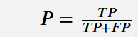
精确率(P)：

从相关结果总量（即真正例TP和假正例FP之和）中正确预测的真正例比例。对于多类别分类问题，精确率在所有类别中取平均值。以下是精确率的公式。

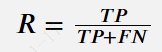
召回率(R)：

从真正例TP和假反例FN的总量中正确预测的真正例比例。对于多类别分类问题，召回率在所有类别中取平均值。以下是召回率的公式。

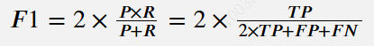
F1分数(F1)：

精确率和召回率的调和平均数。对于多类别分类问题，F1分数在所有类别中取平均值。以下是F1分数的公式。

results = model.evaluate(test_images, verbose=0)

print("    Test Loss: {:.5f}".format(results[0]))
print("Test Accuracy: {:.2f}%".format(results[1] * 100))

输出:

    Test Loss: 0.10042
Test Accuracy: 97.17%

📉可视化损失曲线

accuracy = history.history['accuracy']
val_accuracy = history.history['val_accuracy']

loss = history.history['loss']
val_loss = history.history['val_loss']

epochs = range(len(accuracy))

fig, (ax1, ax2) = plt.subplots(1, 2, figsize=(12, 5))

ax1.plot(epochs, accuracy, 'b', label='Training accuracy')
ax1.plot(epochs, val_accuracy, 'r', label='Validation accuracy')
ax1.set_title('Training and validation accuracy')
ax1.set_xlabel('Epochs')
ax1.set_ylabel('Accuracy')
ax1.legend()

ax2.plot(epochs, loss, 'b', label='Training loss')
ax2.plot(epochs, val_loss, 'r', label='Validation loss')
ax2.set_title('Training and validation loss')
ax2.set_xlabel('Epochs')
ax2.set_ylabel('Loss')
ax2.legend()

fig.suptitle('Training and validation metrics', fontsize=16)
plt.show()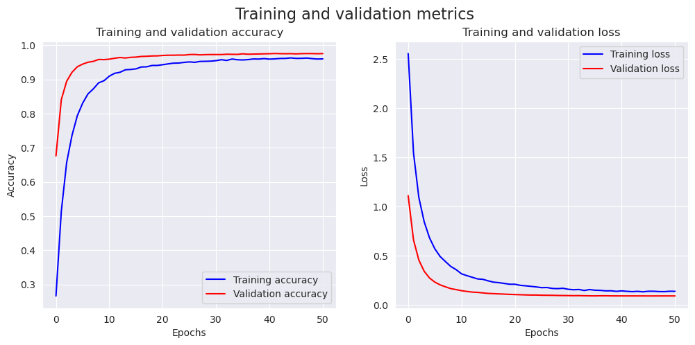

🔮在测试数据上进行预测

#预测测试图像的标签
pred = model.predict(test_images)
pred = np.argmax(pred,axis=1)

# 映射标签
labels = (train_images.class_indices)
labels = dict((v,k) for k,v in labels.items())
pred = [labels[k] for k in pred]

# 显示结果
print(f'The first 5 predictions: {pred[:5]}')

输出:

164/164 [==============================] - 42s 225ms/step
The first 5 predictions: ['cane', 'elefante', 'gallina', 'pecora', 'cane']

 # 从数据集中显示25张随机图片及其标签
random_index = np.random.randint(0, len(test_df) - 1, 15)
fig, axes = plt.subplots(nrows=3, ncols=5, figsize=(25, 15),
                        subplot_kw={'xticks': [], 'yticks': []})

for i, ax in enumerate(axes.flat):
    ax.imshow(plt.imread(test_df.Filepath.iloc[random_index[i]]))
    if test_df.Label.iloc[random_index[i]] == pred[random_index[i]]:
        color = "green"
    else:
        color = "red"
    ax.set_title(f"True: {test_df.Label.iloc[random_index[i]]}\nPredicted: {pred[random_index[i]]}", color=color)
plt.show()
plt.tight_layout()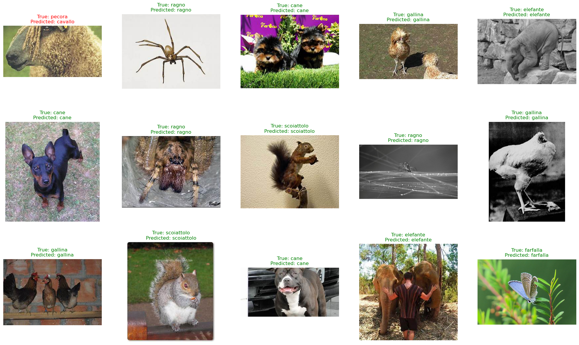

注意: 检测到matplotlib图形，但没有显示数据。可能需要在代码中添加 plt.show() 或确保图像被正确渲染。

<Figure size 640x480 with 0 Axes>

📊绘制分类报告和混淆矩阵

混淆矩阵 和分类报告是用于评估图像分类模型性能的两个重要工具。

混淆矩阵是一个表格，总结了分类模型在测试数据集上做出的正确和错误预测的数量。它通常表示为一个方阵，行和列分别代表预测的类别标签和真实的类别标签。矩阵的条目表示属于某个类别的测试样本数量，以及其中有多少被模型正确或错误分类。混淆矩阵可以提供模型性能的详细分析，包括每个类别的准确率、精确率、召回率和F1分数等指标。它可以用来识别模型在哪些特定区域出现错误，并诊断模型预测的问题。

分类报告是分类模型关键性能指标的总结，包括精确率、召回率和F1分数，以及模型的整体准确率。它提供了模型性能的简明概述，通常按类别细分，可用于快速评估模型的优势和劣势。报告通常以表格形式呈现，每行代表一个类别，列显示各种性能指标。报告还可能包括其他指标，如支持度（属于特定类别的测试样本数量），以及所有类别性能指标的宏观平均值和微观平均值。

在图像分类中，混淆矩阵和分类报告都是评估模型性能、识别改进领域以及决定如何调整模型架构或训练参数的重要工具。

y_test = list(test_df.Label)
print(classification_report(y_test, pred))

输出:

              precision    recall  f1-score   support

        cane       0.97      0.97      0.97       990
     cavallo       0.97      0.96      0.96       568
    elefante       0.99      0.97      0.98       298
    farfalla       0.97      0.97      0.97       390
     gallina       0.99      0.99      0.99       633
       gatto       0.97      0.97      0.97       337
       mucca       0.92      0.94      0.93       379
      pecora       0.94      0.94      0.94       346
       ragno       0.99      0.99      0.99       909
  scoiattolo       0.99      0.99      0.99       376

    accuracy                           0.97      5226
   macro avg       0.97      0.97      0.97      5226
weighted avg       0.97      0.97      0.97      5226

report = classification_report(y_test, pred, output_dict=True)
df = pd.DataFrame(report).transpose()
df

def make_confusion_matrix(y_true, y_pred, classes=None, figsize=(15, 7), text_size=10, norm=False, savefig=False): 
    """创建带有标签的混淆矩阵，比较预测值和真实标签。

    如果传入classes参数，混淆矩阵将使用标签，否则使用整数类别值。

    参数:
      y_true: 真实标签数组（必须与y_pred形状相同）
      y_pred: 预测标签数组（必须与y_true形状相同）
      classes: 类别标签数组（例如字符串形式）。如果为`None`，则使用整数标签
      figsize: 输出图形的大小（默认=(10, 10)）
      text_size: 输出图形文本的大小（默认=15）
      norm: 是否归一化值（默认=False）
      savefig: 是否将混淆矩阵保存到文件（默认=False）
    
    返回:
      比较y_true和y_pred的带标签混淆矩阵图

    使用示例:
      make_confusion_matrix(y_true=test_labels, # 真实测试标签
                            y_pred=y_preds, # 预测标签
                            classes=class_names, # 类别标签名称数组
                            figsize=(15, 15),
                            text_size=10)
    """  
    # 创建混淆矩阵
    cm = confusion_matrix(y_true, y_pred)
    cm_norm = cm.astype("float") / cm.sum(axis=1)[:, np.newaxis] # 归一化
    n_classes = cm.shape[0] # 找出处理的类别数量

    # 绘制图形并美化
    fig, ax = plt.subplots(figsize=figsize)
    cax = ax.matshow(cm, cmap=plt.cm.Blues) # 颜色表示类别的"正确"程度，颜色越深表示越好
    fig.colorbar(cax)

    # 是否有类别列表？
    if classes:
        labels = classes
    else:
        labels = np.arange(cm.shape[0])
  
    # 标注坐标轴
    ax.set(title="混淆矩阵",
           xlabel="预测标签",
           ylabel="真实标签",
           xticks=np.arange(n_classes), # 为每个类别创建足够的轴位置
           yticks=np.arange(n_classes), 
           xticklabels=labels, # 坐标轴将用类别名称（如果存在）或整数标注
           yticklabels=labels)
  
    # 让x轴标签显示在底部
    ax.xaxis.set_label_position("bottom")
    ax.xaxis.tick_bottom()
    ### 新增：旋转xticks以提高可读性并增加字体大小（由于混淆矩阵较大而需要）
    plt.xticks(rotation=90, fontsize=text_size)
    plt.yticks(fontsize=text_size)

    # 设置不同颜色的阈值
    threshold = (cm.max() + cm.min()) / 2.

    # 在每个单元格上绘制文本
    for i, j in itertools.product(range(cm.shape[0]), range(cm.shape[1])):
        if norm:
            plt.text(j, i, f"{cm[i, j]} ({cm_norm[i, j]*100:.1f}%)",
                     horizontalalignment="center",
                     color="white" if cm[i, j] > threshold else "black",
                     size=text_size)
        else:
            plt.text(j, i, f"{cm[i, j]}",
                     horizontalalignment="center",
                     color="white" if cm[i, j] > threshold else "black",
                     size=text_size)

    # 将图形保存到当前工作目录
    if savefig:
        fig.savefig("confusion_matrix.png")

make_confusion_matrix(y_test, pred, list(labels.values()))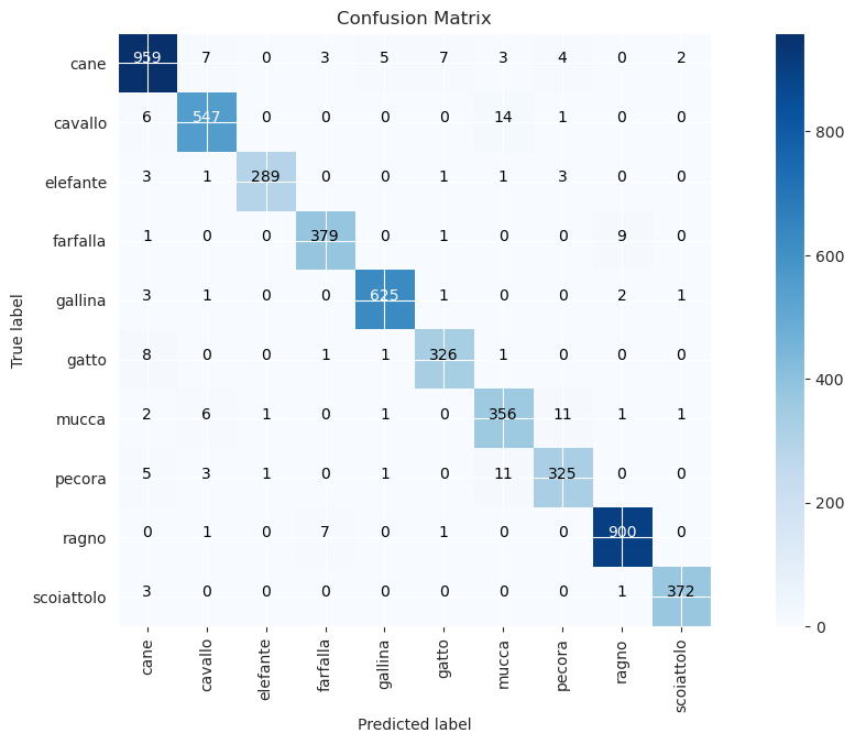

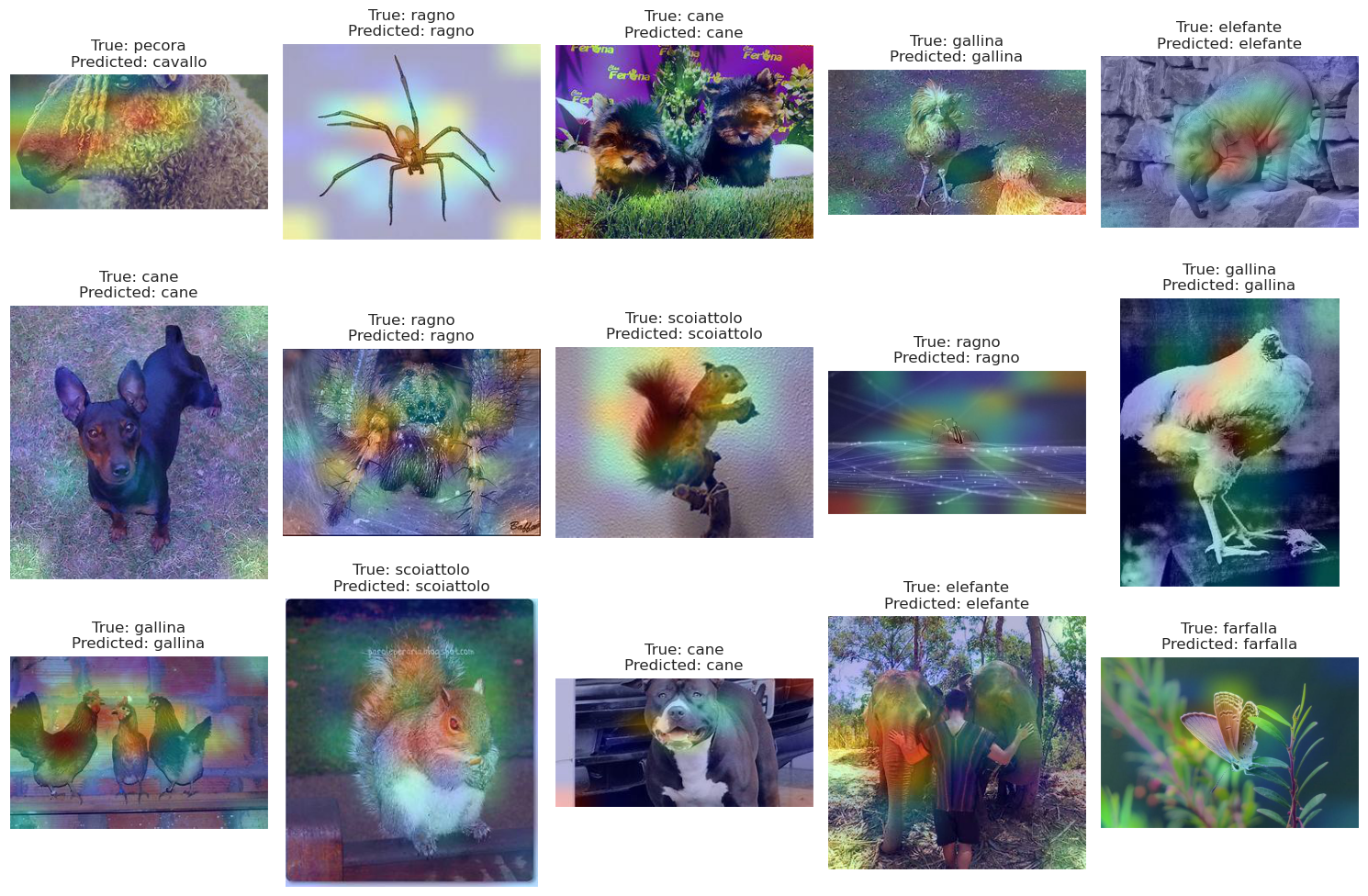
☀️Grad-Cam 可视化

**Grad-CAM（梯度加权类激活映射）**是一种用于可视化输入图像中与神经网络预测最相关区域的技术。它允许您查看模型在做出预测时关注的图像区域。Grad-CAM是CAM技术的改进版本，将其扩展到任何使用卷积神经网络（CNN）作为底层架构的模型。

def get_img_array(img_path, size):
    """加载图像并转换为数组格式"""
    img = tf.keras.preprocessing.image.load_img(img_path, target_size=size)
    array = tf.keras.preprocessing.image.img_to_array(img)
    # 我们添加一个维度将数组转换为指定大小的"批次"
    array = np.expand_dims(array, axis=0)
    return array

def make_gradcam_heatmap(img_array, model, last_conv_layer_name, pred_index=None):
    """生成Grad-CAM热力图"""
    # 首先，我们创建一个模型，将输入图像映射到最后一个卷积层的激活和输出预测
    grad_model = tf.keras.models.Model(
        [model.inputs], [model.get_layer(last_conv_layer_name).output, model.output]
    )

    # 然后，我们计算输入图像的顶部预测类别相对于最后一个卷积层激活的梯度
    with tf.GradientTape() as tape:
        last_conv_layer_output, preds = grad_model(img_array)
        if pred_index is None:
            pred_index = tf.argmax(preds[0])
        class_channel = preds[:, pred_index]
    
    # 这是输出神经元（顶部预测或选择的）相对于最后一个卷积层输出特征图的梯度
    grads = tape.gradient(class_channel, last_conv_layer_output)

    # 这是一个向量，其中每个条目是特定特征图通道上梯度的平均强度
    pooled_grads = tf.reduce_mean(grads, axis=(0, 1, 2))

    # 我们将特征图数组中的每个通道乘以"该通道对于顶部预测类别的重要性"
    # 然后对所有通道求和以获得热力图类别激活
    last_conv_layer_output = last_conv_layer_output[0]
    heatmap = last_conv_layer_output @ pooled_grads[..., tf.newaxis]
    heatmap = tf.squeeze(heatmap)

    # 为了可视化目的，我们还将热力图标准化到0和1之间
    heatmap = tf.maximum(heatmap, 0) / tf.math.reduce_max(heatmap)
    return heatmap.numpy()

def save_and_display_gradcam(img_path, heatmap, cam_path="cam.jpg", alpha=0.4):
    """保存并显示Grad-CAM结果"""
    # 加载原始图像
    img = tf.keras.preprocessing.image.load_img(img_path)
    img = tf.keras.preprocessing.image.img_to_array(img)

    # 将热力图重新缩放到0-255范围
    heatmap = np.uint8(255 * heatmap)

    # 使用jet色彩映射为热力图着色
    jet = cm.get_cmap("jet")

    # 使用色彩映射的RGB值
    jet_colors = jet(np.arange(256))[:, :3]
    jet_heatmap = jet_colors[heatmap]

    # 创建带有RGB彩色热力图的图像
    jet_heatmap = tf.keras.preprocessing.image.array_to_img(jet_heatmap)
    jet_heatmap = jet_heatmap.resize((img.shape[1], img.shape[0]))
    jet_heatmap = tf.keras.preprocessing.image.img_to_array(jet_heatmap)

    # 将热力图叠加到原始图像上
    superimposed_img = jet_heatmap * alpha + img
    superimposed_img = tf.keras.preprocessing.image.array_to_img(superimposed_img)
    
    # 保存叠加后的图像
    superimposed_img.save(cam_path)

    # 显示Grad CAM
    # display(Image(cam_path))
    
    return cam_path
    

preprocess_input = tf.keras.applications.efficientnet.preprocess_input
decode_predictions = tf.keras.applications.efficientnet.decode_predictions

last_conv_layer_name = "top_conv"
img_size = (224, 224, 3)

# 移除最后一层的softmax激活
model.layers[-1].activation = None

# 显示神经网络用于分类的图像区域
fig, axes = plt.subplots(nrows=3, ncols=5, figsize=(15, 10),
                        subplot_kw={'xticks': [], 'yticks': []})

for i, ax in enumerate(axes.flat):
    img_path = test_df.Filepath.iloc[random_index[i]]
    img_array = preprocess_input(get_img_array(img_path, size=img_size))
    heatmap = make_gradcam_heatmap(img_array, model, last_conv_layer_name)
    cam_path = save_and_display_gradcam(img_path, heatmap)
    ax.imshow(plt.imread(cam_path))
    ax.set_title(f"True: {test_df.Label.iloc[random_index[i]]}\nPredicted: {pred[random_index[i]]}")
plt.tight_layout()
plt.show()

代码数据集来源