这篇是为了记录一下,最近学了一下迪哥Ai课堂,听了一下线性回归的理论,用代码简单实现一个线性回归。
工具:jupter
1.引入库以及画图的一个设置
python
import numpy as np
import os
%matplotlib inline
import matplotlib.pyplot as plt
plt.rcParams['axes.labelsize']=14
plt.rcParams['xtick.labelsize']=12
plt.rcParams['ytick.labelsize']=12
import warnings
warnings.filterwarnings('ignore')
2.随机生成一些数据点
python
import numpy as np
X=2*np.random.rand(100,1)
y=4+3*X+np.random.rand(100,1)
plt.plot(X,y,'b.')
plt.xlabel('X_1')
plt.ylabel('y')
plt.axis([0,2,0,15])
plt.show()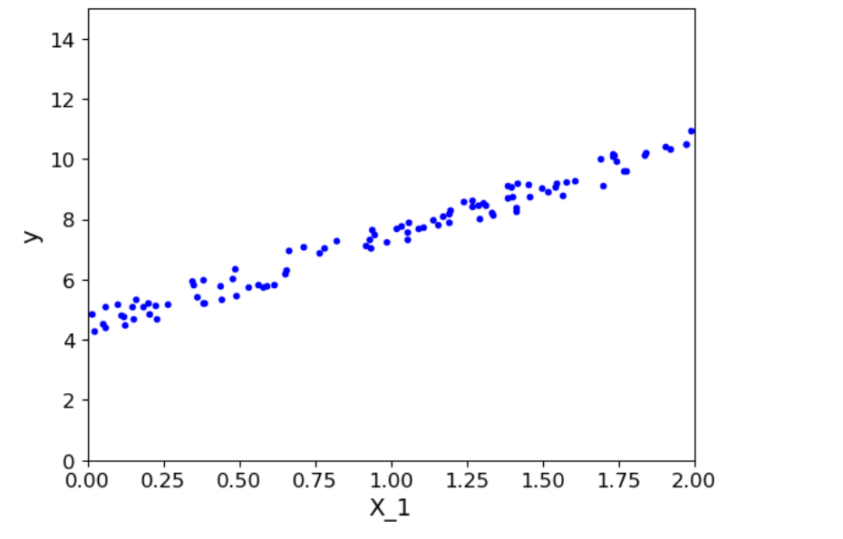
3.添加一列全为1,好计算
python
X_b=np.c_[np.ones((100,1)),X]
X_b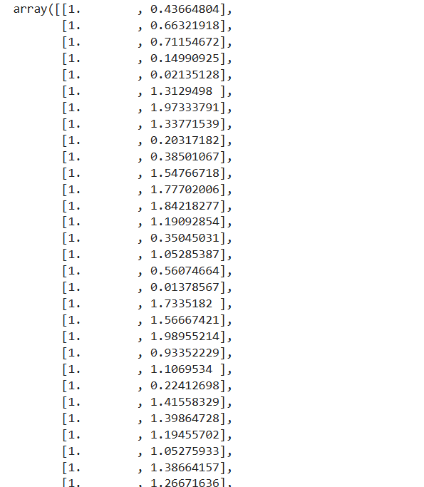
4.代入公式求参数
python
best_theta=np.linalg.inv(X_b.T.dot(X_b)).dot(X_b.T).dot(y)
best_theta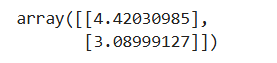
5(1).选择两个数据的x值,来生成预测值,形成一条回归线
python
#选择两个值
X_new=np.array([[0],[2]])
#对它添加一个全为1的列
X_new_b=np.c_[np.ones((2,1)),X_new]
X_new_b
python
#生成预测值
y_pre=X_new_b.dot(best_theta)
y_pre
python
#画图
plt.plot(X_new,y_pre,'r--')
plt.plot(X,y,'b.')
plt.axis([0,2,0,15])
plt.show()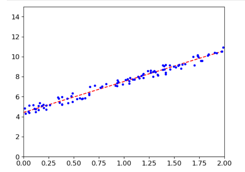
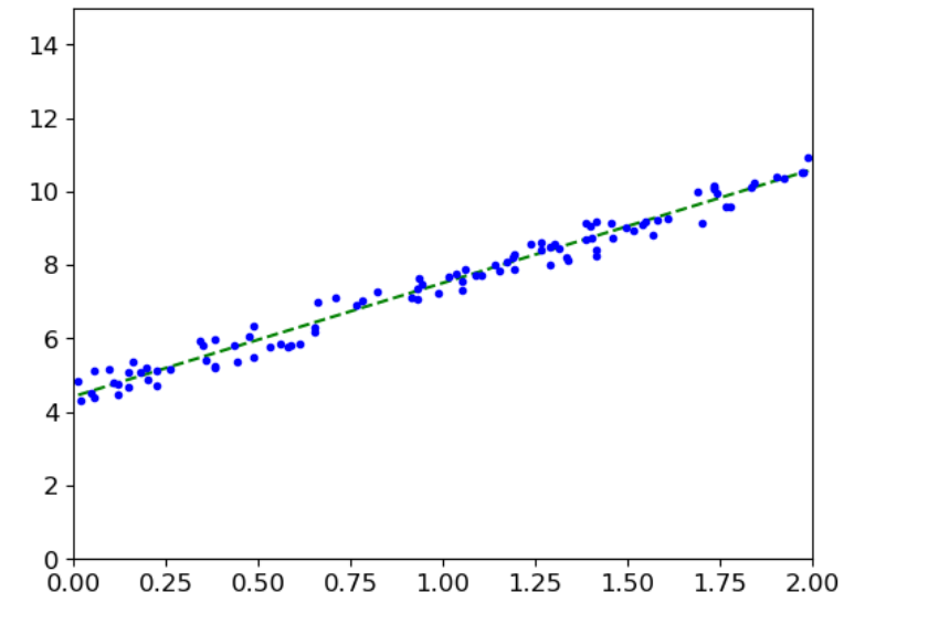
5(2).或者用sklearn库
python
from sklearn.linear_model import LinearRegression
#实例化
lin_reg=LinearRegression()
#训练学习x,y
lin_reg.fit(X,y)
#斜率
print(lin_reg.coef_)
#截距
print(lin_reg.intercept_)
python
#用上面选择的两个点的x值进行测试
y_pred = lin_reg.predict(X_new)
#画图
plt.plot(X_new,y_pred,'g--')
plt.plot(X,y,'b.')
plt.axis([0,2,0,15])
plt.show()
也能得到这个结果
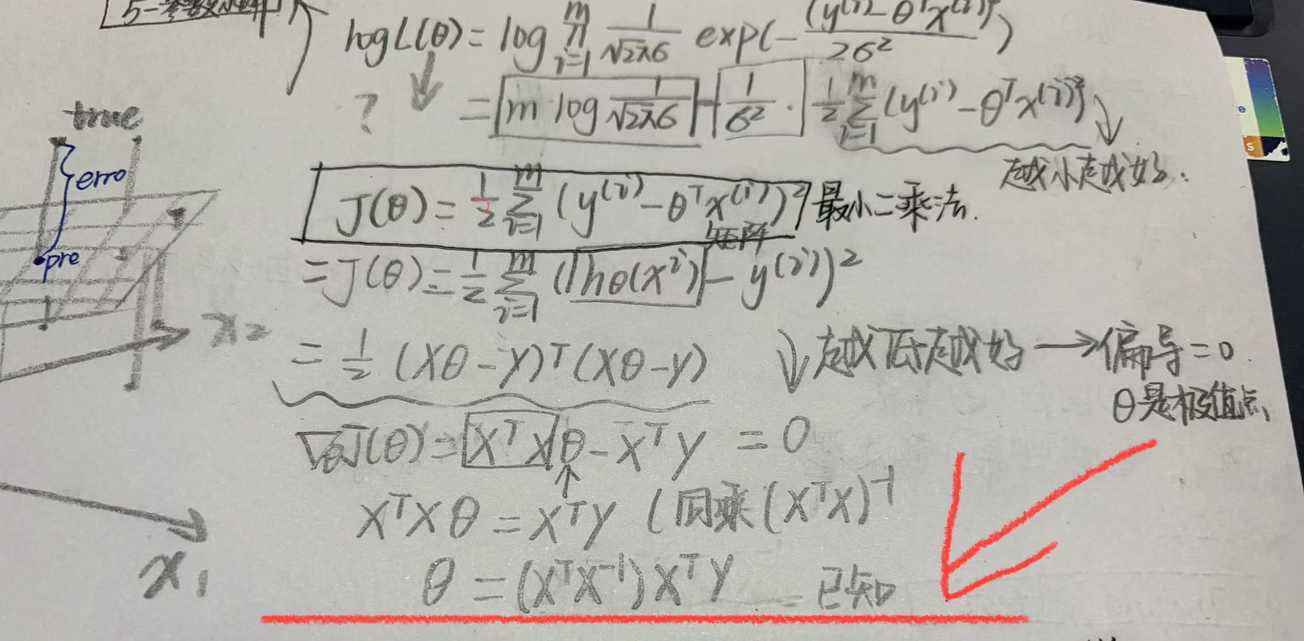
6.梯度下降
线性回归定义了需要解决的问题(目标和模型),而梯度下降是解决这个问题的关键方法(优化算法)。线性回归的目标是找到一组最佳的参数(w 和 b ),使得模型的预测值 y_pred与真实值 y_true之间的差距最小,即损失函数。
损失函数 :为了衡量这个"差距",我们定义一个函数,最常见的是均方误差:
MSE Loss = (1/m) * Σ(y_true - y_pred)²其中
m是样本数量。这个函数计算了所有预测误差的平方的平均值。我们的目标就是找到让MSE Loss值最小的那组 w 和 b。
所以,线性回归问题就转化为了一个数学优化问题 :寻找使损失函数最小化的参数。
6(1).批量梯度下降
python
#批量梯度下降
eta = 0.1
n_iterations=1000
m=100
theta =np.random.randn(2,1)
for iteration in range(n_iterations):
    gradients=2/m*X_b.T.dot(X_b.dot(theta)-y)
    theta =theta-eta*gradients
X_new_b.dot(theta)
theta_path_bgd = []
def plot_gradient_descent(theta,eta,theta_path=None):
    m=len(X_b)
    plt.plot(X,y,'b.')
    n_iterations=1000
    for iteration in range(n_iterations):
        y_predict =X_new_b.dot(theta)
        plt.plot(X_new,y_predict,'b--')
        gradients=2/m*X_b.T.dot(X_b.dot(theta)-y)
        theta =theta-eta*gradients
        if theta_path is not None:
            theta_path_bgd.append(theta)
    plt.xlabel('X_1')
    plt.axis([0,2,0,15])
    plt.title('eta={}'.format(eta))
theta = np.random.randn(2,1)
plt.figure(figsize=(10,4))
plt.subplot(131)
plot_gradient_descent(theta,eta=0.02)
plt.subplot(132)
plot_gradient_descent(theta,eta=0.1,theta_path=theta_path_bgd)
plt.subplot(133)
plot_gradient_descent(theta,eta=0.5)
plt.show()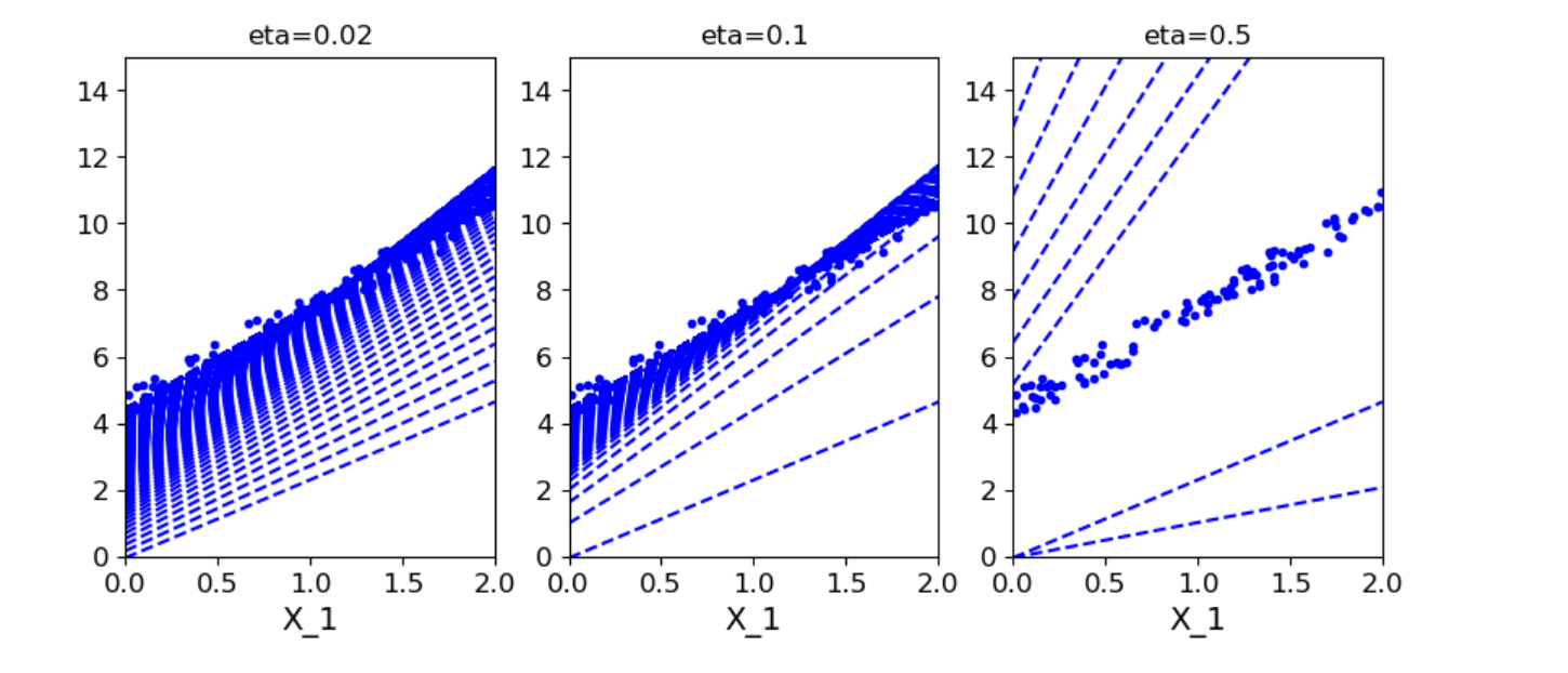
6(2).随机梯度下降
python
#随机梯度下降
theta_path_sgd=[]
m= len(X_b)
n_epochs=50

t0=5
t1=50

def learning_schedule(t):
    return t0/(t1+t)

theta= np.random.randn(2,1)
for epoch in range(n_epochs):
    for i in range(m):
        if epoch <10 and i<10:
             y_predict =X_new_b.dot(theta)
             plt.plot(X_new,y_predict,'r--')
        random_index = np.random.randint(m)
        xi=X_b[random_index:random_index+1]
        yi=y[random_index:random_index+1]
        gradients=2*xi.T.dot(xi.dot(theta)-yi)
        eta=learning_schedule(n_epochs*m+i)
        theta = theta-eta*gradients
        theta_path_sgd.append(theta)


plt.axis([0,2,0,15])
plt.plot(X,y,'b.')
plt.show()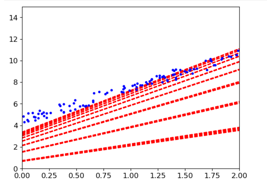
6(3)小批量梯度下降
python
#小批量梯度下降
theta_path_mgd=[]
n_iterations=50
minibatch=16
theta = np.random.randn(2,1)
t=0
for epoch  in range(n_epochs):
    shuffled_indices = np.random.permutation(m)
    X_b_shuffled=X_b[shuffled_indices]
    y_shuffled = y[shuffled_indices]
    for i in range(0,m,minibatch):
        t+=1
        xi=X_b_shuffled[i:i+minibatch]
        yi=y_shuffled[i:i+minibatch]
        gradients=2/minibatch*xi.T.dot(xi.dot(theta)-yi)
        eta=learning_schedule(t)
        theta = theta-eta*gradients
        theta_path_mgd.append(theta)
        if epoch <10 and i<10:
             y_predict =X_new_b.dot(theta)
             plt.plot(X_new,y_predict,'r--')

plt.axis([0,2,0,15])
plt.plot(X,y,'b.')
plt.show()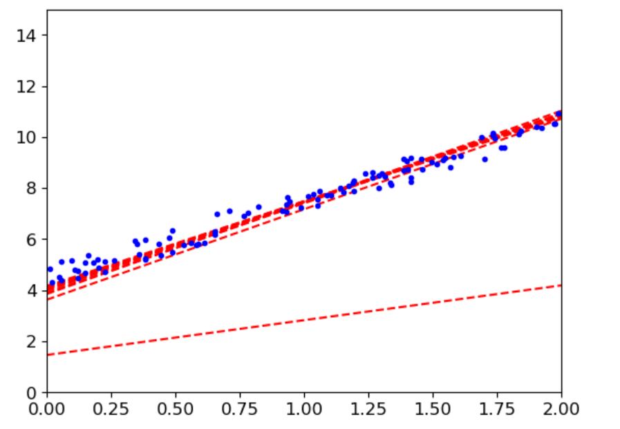
6.对比
python
theta_path_bgd=np.array(theta_path_bgd)
theta_path_sgd=np.array(theta_path_sgd)
theta_path_mgd=np.array(theta_path_mgd)
plt.figure(figsize=(8,4))
plt.plot(theta_path_sgd[:,0],theta_path_sgd[:,1],'r-s',linewidth=1,label='SGD')
plt.plot(theta_path_mgd[:,0],theta_path_mgd[:,1],'g-+',linewidth=2,label='mini')
plt.plot(theta_path_bgd[:,0],theta_path_bgd[:,1],'b-o',linewidth=3,label='BGD')
plt.legend(loc='upper left')
plt.axis([3.5,4.5,2.0,4.0])
plt.show()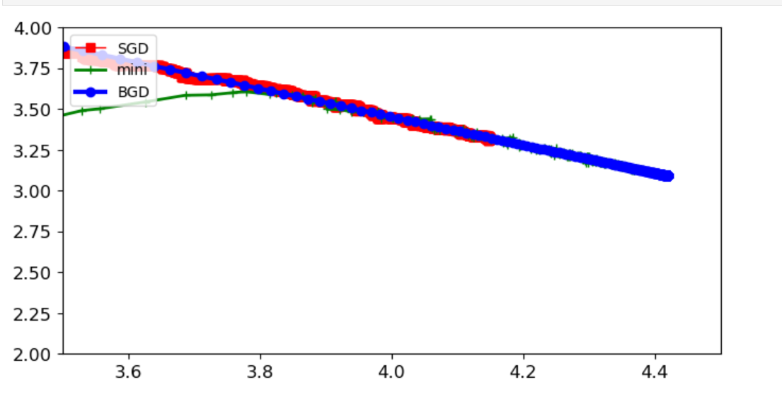
-
BGD(批量梯度下降):收敛稳定但慢,适合小数据集
-
SGD(随机梯度下降):收敛快但波动大,需要学习率调度
-
Mini-batch(小批量梯度下降):实践中最常用,兼顾效率和稳定性
好不容易理解了一点理论,结果发现写成python逻辑就乱成一团浆糊了,累了,等下一次感兴趣在研究吧。