day27pipeline管道@浙大疏锦行
| Id | Home Ownership | Annual Income | Years in current job | Tax Liens | Number of Open Accounts | Years of Credit History | Maximum Open Credit | Number of Credit Problems | Months since last delinquent | Bankruptcies | Purpose | Term | Current Loan Amount | Current Credit Balance | Monthly Debt | Credit Score | Credit Default | |
|---|---|---|---|---|---|---|---|---|---|---|---|---|---|---|---|---|---|---|
| 0 | 0 | Own Home | 482087.0 | NaN | 0.0 | 11.0 | 26.3 | 685960.0 | 1.0 | NaN | 1.0 | debt consolidation | Short Term | 99999999.0 | 47386.0 | 7914.0 | 749.0 | 0 |
| 1 | 1 | Own Home | 1025487.0 | 10+ years | 0.0 | 15.0 | 15.3 | 1181730.0 | 0.0 | NaN | 0.0 | debt consolidation | Long Term | 264968.0 | 394972.0 | 18373.0 | 737.0 | 1 |
| 2 | 2 | Home Mortgage | 751412.0 | 8 years | 0.0 | 11.0 | 35.0 | 1182434.0 | 0.0 | NaN | 0.0 | debt consolidation | Short Term | 99999999.0 | 308389.0 | 13651.0 | 742.0 | 0 |
| 3 | 3 | Own Home | 805068.0 | 6 years | 0.0 | 8.0 | 22.5 | 147400.0 | 1.0 | NaN | 1.0 | debt consolidation | Short Term | 121396.0 | 95855.0 | 11338.0 | 694.0 | 0 |
| 4 | 4 | Rent | 776264.0 | 8 years | 0.0 | 13.0 | 13.6 | 385836.0 | 1.0 | NaN | 0.0 | debt consolidation | Short Term | 125840.0 | 93309.0 | 7180.0 | 719.0 | 0 |
1. 特征类型分类配置
根据数据特点,将特征分为:
-
有序分类特征:有明确顺序关系的分类特征(如工作年限)
-
标称分类特征:无顺序关系的分类特征(如贷款目的)
-
数值特征:连续数值特征
python
# ==========================================
# 特征配置(适用于当前数据集,可根据实际数据调整)
# ==========================================

# 目标变量
TARGET = 'Credit Default'

# 分离特征和标签
y = data[TARGET]
X = data.drop([TARGET], axis=1)

# ---------- 有序分类特征配置 ----------
# 定义有序分类特征及其类别顺序
ordinal_features = ['Home Ownership', 'Years in current job', 'Term']

# 每个有序特征的类别顺序(编码顺序:0, 1, 2, ...)
ordinal_categories = [
    ['Own Home', 'Rent', 'Have Mortgage', 'Home Mortgage'],  # Home Ownership
    ['< 1 year', '1 year', '2 years', '3 years', '4 years', '5 years',
     '6 years', '7 years', '8 years', '9 years', '10+ years'],  # Years in current job
    ['Short Term', 'Long Term']  # Term
]

# ---------- 标称分类特征配置 ----------
# 需要独热编码的特征
nominal_features = ['Purpose']

# ---------- 数值特征配置 ----------
# 自动识别:排除分类特征后的所有列
all_categorical = ordinal_features + nominal_features
numeric_features = [col for col in X.columns if col not in all_categorical]

print("=" * 60)
print("特征类型配置")
print("=" * 60)
print(f"目标变量: {TARGET}")
print(f"\n有序分类特征 ({len(ordinal_features)}个): {ordinal_features}")
print(f"\n标称分类特征 ({len(nominal_features)}个): {nominal_features}")
print(f"\n数值特征 ({len(numeric_features)}个): {numeric_features}")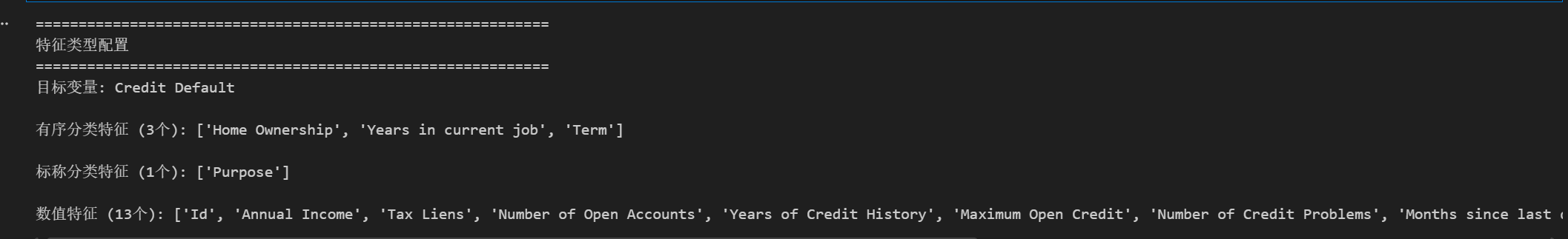
2. 构建通用预处理 Pipeline
使用 ColumnTransformer 将不同的预处理步骤应用于不同类型的特征:
-
有序特征:众数填充 + OrdinalEncoder
-
标称特征:众数填充 + OneHotEncoder
-
数值特征:众数填充 + StandardScaler
python
# ==========================================
# 构建预处理器(ColumnTransformer)
# ==========================================

# 有序特征处理器:众数填充 + 有序编码
ordinal_transformer = Pipeline(steps=[
    ('imputer', SimpleImputer(strategy='most_frequent')),
    ('encoder', OrdinalEncoder(
        categories=ordinal_categories,
        handle_unknown='use_encoded_value',
        unknown_value=-1
    ))
])

# 标称特征处理器:众数填充 + 独热编码
nominal_transformer = Pipeline(steps=[
    ('imputer', SimpleImputer(strategy='most_frequent')),
    ('onehot', OneHotEncoder(handle_unknown='ignore', sparse_output=False))
])

# 数值特征处理器:众数填充 + 标准化
numeric_transformer = Pipeline(steps=[
    ('imputer', SimpleImputer(strategy='most_frequent')),
    ('scaler', StandardScaler())
])

# 组合所有预处理器
preprocessor = ColumnTransformer(
    transformers=[
        ('ordinal', ordinal_transformer, ordinal_features),
        ('nominal', nominal_transformer, nominal_features),
        ('numeric', numeric_transformer, numeric_features)
    ],
    remainder='drop'  # 丢弃未指定的列
)

print("✅ 预处理器构建完成!")
print("\n预处理器结构:")
print(preprocessor)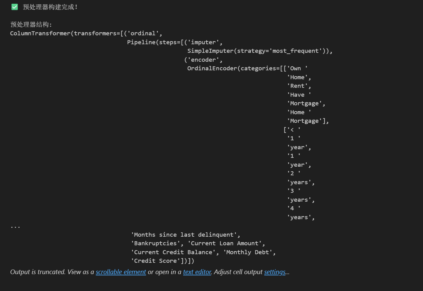
3. 定义模型字典
定义一个包含多种机器学习模型的字典,方便后续批量训练和比较
python
# ==========================================
# 定义多种机器学习模型
# ==========================================

# 模型字典:模型名称 -> (模型实例, 参数网格)
# 参数网格用于网格搜索调参,格式为 {'pipeline参数名': [候选值列表]}
# 注意:在Pipeline中,参数名格式为 'step_name__parameter_name'

models = {
    '随机森林': {
        'model': RandomForestClassifier(random_state=42),
        'params': {
            'classifier__n_estimators': [100, 200],
            'classifier__max_depth': [10, 20, None],
            'classifier__min_samples_split': [2, 5]
        }
    },
    'XGBoost': {
        'model': XGBClassifier(random_state=42, eval_metric='logloss'),
        'params': {
            'classifier__n_estimators': [100, 200],
            'classifier__max_depth': [3, 6, 9],
            'classifier__learning_rate': [0.01, 0.1]
        }
    },
    'LightGBM': {
        'model': LGBMClassifier(random_state=42, verbosity=-1),
        'params': {
            'classifier__n_estimators': [100, 200],
            'classifier__max_depth': [3, 6, -1],
            'classifier__learning_rate': [0.01, 0.1]
        }
    },
    '逻辑回归': {
        'model': LogisticRegression(random_state=42, max_iter=1000),
        'params': {
            'classifier__C': [0.01, 0.1, 1, 10],
            'classifier__penalty': ['l2']
        }
    },
    'SVM': {
        'model': SVC(random_state=42, probability=True),
        'params': {
            'classifier__C': [0.1, 1, 10],
            'classifier__kernel': ['rbf', 'linear']
        }
    },
    'KNN': {
        'model': KNeighborsClassifier(),
        'params': {
            'classifier__n_neighbors': [3, 5, 7],
            'classifier__weights': ['uniform', 'distance']
        }
    },
    '决策树': {
        'model': DecisionTreeClassifier(random_state=42),
        'params': {
            'classifier__max_depth': [5, 10, 20, None],
            'classifier__min_samples_split': [2, 5, 10]
        }
    },
    '梯度提升': {
        'model': GradientBoostingClassifier(random_state=42),
        'params': {
            'classifier__n_estimators': [100, 200],
            'classifier__max_depth': [3, 5],
            'classifier__learning_rate': [0.01, 0.1]
        }
    }
}

print(f"✅ 已定义 {len(models)} 种机器学习模型!")
for name in models.keys():
    print(f"   - {name}")
4. 划分数据集
python
# ==========================================
# 划分训练集和测试集(在预处理之前划分,防止数据泄露)
# ==========================================

X_train, X_test, y_train, y_test = train_test_split(
    X, y,
    test_size=0.2,
    random_state=42,
    stratify=y  # 分层采样,保持类别比例一致
)

print("=" * 60)
print("数据集划分完成")
print("=" * 60)
print(f"训练集: {X_train.shape[0]} 样本")
print(f"测试集: {X_test.shape[0]} 样本")
print(f"\n训练集目标分布:\n{y_train.value_counts()}")
print(f"\n测试集目标分布:\n{y_test.value_counts()}")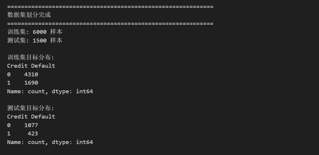
5. 创建通用 Pipeline 构建函数
python
# ==========================================
# 通用 Pipeline 构建函数
# ==========================================

def create_pipeline(model, preprocessor):
    """
    创建完整的机器学习 Pipeline

    参数:
        model: sklearn 模型实例
        preprocessor: ColumnTransformer 预处理器

    返回:
        Pipeline 对象
    """
    return Pipeline(steps=[
        ('preprocessor', preprocessor),
        ('classifier', model)
    ])


def evaluate_model(pipeline, X_train, X_test, y_train, y_test, model_name="模型"):
    """
    训练并评估模型

    参数:
        pipeline: Pipeline 对象
        X_train, X_test: 训练集和测试集特征
        y_train, y_test: 训练集和测试集标签
        model_name: 模型名称(用于打印)

    返回:
        dict: 包含各种评估指标的字典
    """
    start_time = time.time()

    # 训练模型
    pipeline.fit(X_train, y_train)

    # 预测
    y_pred = pipeline.predict(X_test)
    y_pred_proba = pipeline.predict_proba(X_test)[:, 1] if hasattr(pipeline, 'predict_proba') else None

    train_time = time.time() - start_time

    # 计算评估指标
    results = {
        'model_name': model_name,
        'accuracy': accuracy_score(y_test, y_pred),
        'precision': precision_score(y_test, y_pred),
        'recall': recall_score(y_test, y_pred),
        'f1': f1_score(y_test, y_pred),
        'roc_auc': roc_auc_score(y_test, y_pred_proba) if y_pred_proba is not None else None,
        'train_time': train_time,
        'pipeline': pipeline,
        'y_pred': y_pred,
        'y_pred_proba': y_pred_proba
    }

    return results


def print_evaluation_report(results):
    """打印评估报告"""
    print(f"\n{'='*60}")
    print(f"模型: {results['model_name']}")
    print(f"{'='*60}")
    print(f"训练耗时: {results['train_time']:.4f} 秒")
    print(f"\n评估指标:")
    print(f"  准确率 (Accuracy):  {results['accuracy']:.4f}")
    print(f"  精确率 (Precision): {results['precision']:.4f}")
    print(f"  召回率 (Recall):    {results['recall']:.4f}")
    print(f"  F1 分数:            {results['f1']:.4f}")
    if results['roc_auc']:
        print(f"  AUC-ROC:            {results['roc_auc']:.4f}")


print("✅ 通用函数定义完成!")
6. 批量训练和评估所有模型(使用默认参数)
python
# ==========================================
# 批量训练和评估所有模型
# ==========================================

all_results = []

print("开始训练所有模型...")
print("=" * 80)

for model_name, model_config in models.items():
    # 创建 Pipeline
    pipeline = create_pipeline(model_config['model'], preprocessor)

    # 训练和评估
    results = evaluate_model(pipeline, X_train, X_test, y_train, y_test, model_name)
    all_results.append(results)

    # 打印简要结果
    auc_str = f"{results['roc_auc']:.4f}" if results['roc_auc'] else 'N/A'
    print(f"{model_name:12s} | 准确率: {results['accuracy']:.4f} | F1: {results['f1']:.4f} | AUC: {auc_str} | 耗时: {results['train_time']:.2f}s")

print("=" * 80)
print("✅ 所有模型训练完成!")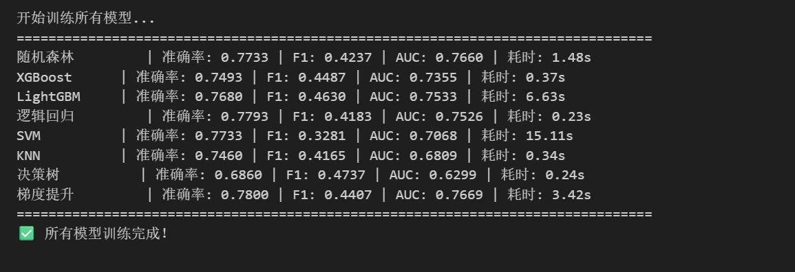
7. 模型对比可视化
python
# ==========================================
# 模型性能对比可视化
# ==========================================
# 将结果转换为DataFrame
results_df = pd.DataFrame([{
'模型': r['model_name'],
'准确率': r['accuracy'],
'精确率': r['precision'],
'召回率': r['recall'],
'F1分数': r['f1'],
'AUC-ROC': r['roc_auc'],
'训练时间(s)': r['train_time']
} for r in all_results])
# 按F1分数排序
results_df = results_df.sort_values('F1分数', ascending=False)
print("模型性能对比表(按F1分数排序):")
display(results_df)
# 绘制对比图
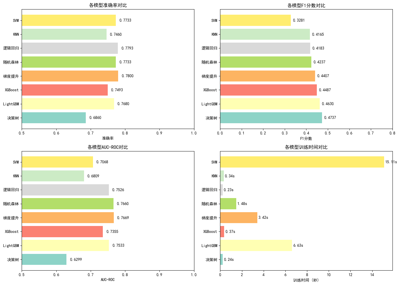
fig, axes = plt.subplots(2, 2, figsize=(14, 10))
# 1. 准确率对比
ax1 = axes[0, 0]
colors = plt.cm.Set3(np.linspace(0, 1, len(results_df)))
bars1 = ax1.barh(results_df['模型'], results_df['准确率'], color=colors)
ax1.set_xlabel('准确率')
ax1.set_title('各模型准确率对比')
ax1.set_xlim([0.5, 1.0])
for bar, val in zip(bars1, results_df['准确率']):
ax1.text(val + 0.01, bar.get_y() + bar.get_height()/2, f'{val:.4f}', va='center')
# 2. F1分数对比
ax2 = axes[0, 1]
bars2 = ax2.barh(results_df['模型'], results_df['F1分数'], color=colors)
ax2.set_xlabel('F1分数')
ax2.set_title('各模型F1分数对比')
ax2.set_xlim([0, 0.8])
for bar, val in zip(bars2, results_df['F1分数']):
ax2.text(val + 0.01, bar.get_y() + bar.get_height()/2, f'{val:.4f}', va='center')
# 3. AUC-ROC对比
ax3 = axes[1, 0]
bars3 = ax3.barh(results_df['模型'], results_df['AUC-ROC'], color=colors)
ax3.set_xlabel('AUC-ROC')
ax3.set_title('各模型AUC-ROC对比')
ax3.set_xlim([0.5, 1.0])
for bar, val in zip(bars3, results_df['AUC-ROC']):
ax3.text(val + 0.01, bar.get_y() + bar.get_height()/2, f'{val:.4f}', va='center')
# 4. 训练时间对比
ax4 = axes[1, 1]
bars4 = ax4.barh(results_df['模型'], results_df['训练时间(s)'], color=colors)
ax4.set_xlabel('训练时间 (秒)')
ax4.set_title('各模型训练时间对比')
for bar, val in zip(bars4, results_df['训练时间(s)']):
ax4.text(val + 0.1, bar.get_y() + bar.get_height()/2, f'{val:.2f}s', va='center')
plt.tight_layout()
plt.savefig('model_comparison.png', dpi=150, bbox_inches='tight')
plt.show()
print("\n✅ 对比图已保存为 model_comparison.png")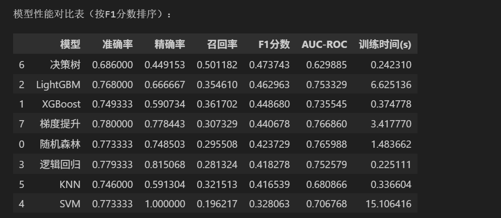
8. ROC曲线对比
python
# ==========================================
# ROC曲线对比
# ==========================================

plt.figure(figsize=(10, 8))

# 绘制每个模型的ROC曲线
for result in all_results:
    if result['y_pred_proba'] is not None:
        fpr, tpr, _ = roc_curve(y_test, result['y_pred_proba'])
        auc = result['roc_auc']
        plt.plot(fpr, tpr, label=f"{result['model_name']} (AUC={auc:.4f})", linewidth=2)

# 绘制对角线(随机分类器)
plt.plot([0, 1], [0, 1], 'k--', label='随机分类器', linewidth=1)

plt.xlabel('假阳性率 (FPR)', fontsize=12)
plt.ylabel('真阳性率 (TPR)', fontsize=12)
plt.title('各模型ROC曲线对比', fontsize=14)
plt.legend(loc='lower right', fontsize=10)
plt.grid(True, alpha=0.3)

plt.tight_layout()
plt.savefig('roc_curves.png', dpi=150, bbox_inches='tight')
plt.show()

print("\n✅ ROC曲线图已保存为 roc_curves.png")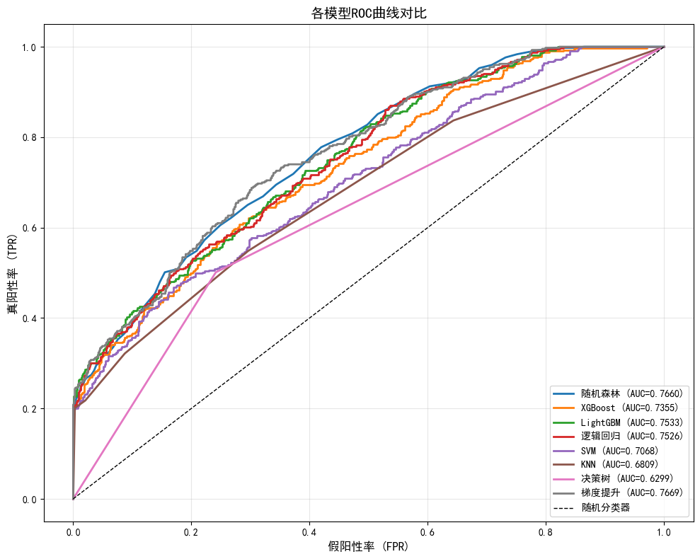
9. 选择最佳模型并进行详细评估
python
# ==========================================
# 选择最佳模型(按AUC-ROC)
# ==========================================
# 找到AUC最高的模型
best_result = max(all_results, key=lambda x: x['roc_auc'] if x['roc_auc'] else 0)
best_model_name = best_result['model_name']
best_pipeline = best_result['pipeline']
print("=" * 60)
print(f"最佳模型: {best_model_name}")
print("=" * 60)
# 详细评估报告
print_evaluation_report(best_result)
# 分类报告
print(f"\n详细分类报告:")
print(classification_report(y_test, best_result['y_pred']))
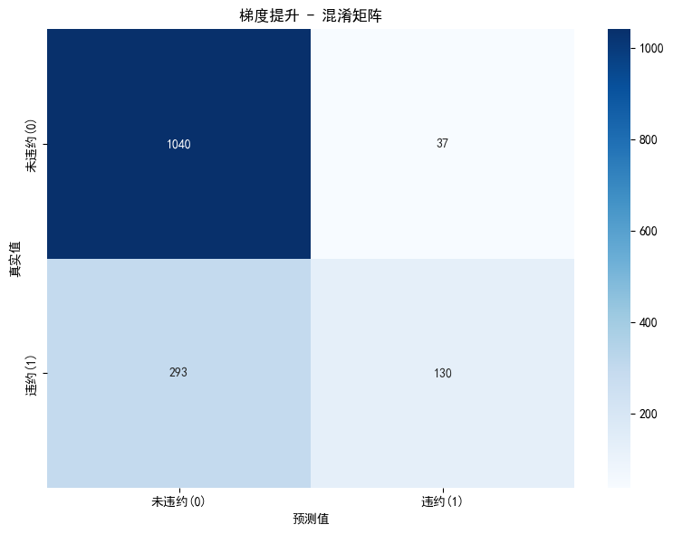
# 混淆矩阵可视化
plt.figure(figsize=(8, 6))
cm = confusion_matrix(y_test, best_result['y_pred'])
sns.heatmap(cm, annot=True, fmt='d', cmap='Blues',
xticklabels=['未违约(0)', '违约(1)'],
yticklabels=['未违约(0)', '违约(1)'])
plt.xlabel('预测值')
plt.ylabel('真实值')
plt.title(f'{best_model_name} - 混淆矩阵')
plt.tight_layout()
plt.savefig('best_model_confusion_matrix.png', dpi=150, bbox_inches='tight')
plt.show()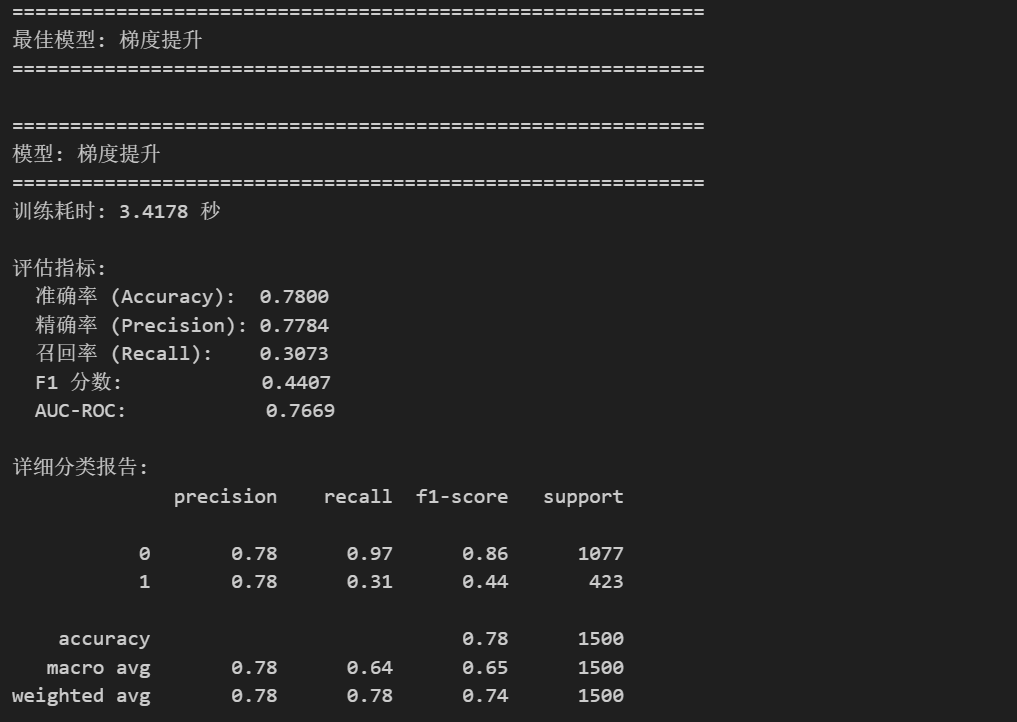
10. 使用网格搜索进行超参数调优(以随机森林为例)
python
# ==========================================
# 网格搜索调参示例(以梯度提升为例,因为它是当前最佳模型)
# ==========================================

print("开始网格搜索调参...")
print("=" * 60)

# 创建Pipeline
tuning_pipeline = create_pipeline(GradientBoostingClassifier(random_state=42), preprocessor)

# 定义参数网格(简化版,避免过长时间)
param_grid = {
    'classifier__n_estimators': [100, 150, 200],
    'classifier__max_depth': [3, 5, 7],
    'classifier__learning_rate': [0.05, 0.1, 0.15]
}

# 创建网格搜索对象
grid_search = GridSearchCV(
    tuning_pipeline,
    param_grid,
    cv=5,                    # 5折交叉验证
    scoring='roc_auc',       # 使用AUC-ROC作为评分指标
    n_jobs=-1,               # 使用所有CPU核心
    verbose=1
)

# 执行网格搜索
start_time = time.time()
grid_search.fit(X_train, y_train)
grid_time = time.time() - start_time

print(f"\n网格搜索完成!耗时: {grid_time:.2f} 秒")
print(f"\n最佳参数: {grid_search.best_params_}")
print(f"最佳交叉验证AUC: {grid_search.best_score_:.4f}")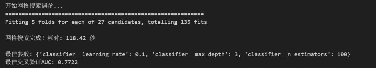
python
# ==========================================
# 使用最佳参数的模型在测试集上评估
# ==========================================

# 获取最佳模型
best_tuned_pipeline = grid_search.best_estimator_

# 在测试集上预测
y_pred_tuned = best_tuned_pipeline.predict(X_test)
y_pred_proba_tuned = best_tuned_pipeline.predict_proba(X_test)[:, 1]

# 计算评估指标
print("=" * 60)
print("调参后的梯度提升模型 - 测试集表现")
print("=" * 60)
print(f"准确率 (Accuracy):  {accuracy_score(y_test, y_pred_tuned):.4f}")
print(f"精确率 (Precision): {precision_score(y_test, y_pred_tuned):.4f}")
print(f"召回率 (Recall):    {recall_score(y_test, y_pred_tuned):.4f}")
print(f"F1 分数:            {f1_score(y_test, y_pred_tuned):.4f}")
print(f"AUC-ROC:            {roc_auc_score(y_test, y_pred_proba_tuned):.4f}")

print("\n详细分类报告:")
print(classification_report(y_test, y_pred_tuned))

# 与调参前对比
print("\n" + "=" * 60)
print("调参前后对比")
print("=" * 60)
original_auc = [r['roc_auc'] for r in all_results if r['model_name'] == '梯度提升'][0]
tuned_auc = roc_auc_score(y_test, y_pred_proba_tuned)
print(f"默认参数 AUC-ROC: {original_auc:.4f}")
print(f"调参后 AUC-ROC:   {tuned_auc:.4f}")
print(f"提升:             {(tuned_auc - original_auc) * 100:.2f}%")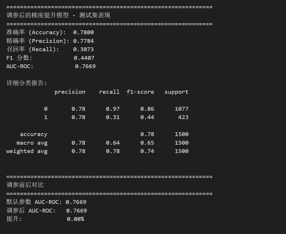
11. 通用 Pipeline 封装类
将整个流程封装成一个可复用的类,方便在其他项目中使用
python
# ==========================================
# 通用机器学习 Pipeline 封装类
# ==========================================

class UniversalMLPipeline:
    """
    通用机器学习 Pipeline 类

    功能:
    1. 自动识别和处理不同类型的特征
    2. 支持多种机器学习模型
    3. 支持网格搜索调参
    4. 提供完整的评估报告
    """

    def __init__(self,
                 ordinal_features=None,
                 ordinal_categories=None,
                 nominal_features=None,
                 numeric_features=None,
                 impute_strategy='most_frequent',
                 scale_numeric=True):
        """
        初始化 Pipeline

        参数:
            ordinal_features: 有序分类特征列表
            ordinal_categories: 有序分类特征的类别顺序
            nominal_features: 标称分类特征列表
            numeric_features: 数值特征列表(如果为None,则自动识别)
            impute_strategy: 缺失值填充策略 ('most_frequent', 'mean', 'median')
            scale_numeric: 是否对数值特征进行标准化
        """
        self.ordinal_features = ordinal_features or []
        self.ordinal_categories = ordinal_categories or []
        self.nominal_features = nominal_features or []
        self.numeric_features = numeric_features
        self.impute_strategy = impute_strategy
        self.scale_numeric = scale_numeric

        self.preprocessor = None
        self.pipeline = None
        self.results = {}

    def _build_preprocessor(self, X):
        """构建预处理器"""
        # 自动识别数值特征
        if self.numeric_features is None:
            all_categorical = self.ordinal_features + self.nominal_features
            self.numeric_features = [col for col in X.columns if col not in all_categorical]

        transformers = []

        # 有序特征处理
        if self.ordinal_features:
            ordinal_transformer = Pipeline(steps=[
                ('imputer', SimpleImputer(strategy='most_frequent')),
                ('encoder', OrdinalEncoder(
                    categories=self.ordinal_categories,
                    handle_unknown='use_encoded_value',
                    unknown_value=-1
                ))
            ])
            transformers.append(('ordinal', ordinal_transformer, self.ordinal_features))

        # 标称特征处理
        if self.nominal_features:
            nominal_transformer = Pipeline(steps=[
                ('imputer', SimpleImputer(strategy='most_frequent')),
                ('onehot', OneHotEncoder(handle_unknown='ignore', sparse_output=False))
            ])
            transformers.append(('nominal', nominal_transformer, self.nominal_features))

        # 数值特征处理
        if self.numeric_features:
            steps = [('imputer', SimpleImputer(strategy=self.impute_strategy))]
            if self.scale_numeric:
                steps.append(('scaler', StandardScaler()))
            numeric_transformer = Pipeline(steps=steps)
            transformers.append(('numeric', numeric_transformer, self.numeric_features))

        self.preprocessor = ColumnTransformer(
            transformers=transformers,
            remainder='drop'
        )

        return self.preprocessor

    def create_pipeline(self, model):
        """创建完整的 Pipeline"""
        return Pipeline(steps=[
            ('preprocessor', self.preprocessor),
            ('classifier', model)
        ])

    def fit_evaluate(self, X_train, X_test, y_train, y_test, model, model_name="模型"):
        """训练并评估模型"""
        if self.preprocessor is None:
            self._build_preprocessor(X_train)

        pipeline = self.create_pipeline(model)

        start_time = time.time()
        pipeline.fit(X_train, y_train)

        y_pred = pipeline.predict(X_test)
        y_pred_proba = pipeline.predict_proba(X_test)[:, 1] if hasattr(pipeline, 'predict_proba') else None

        train_time = time.time() - start_time

        results = {
            'model_name': model_name,
            'accuracy': accuracy_score(y_test, y_pred),
            'precision': precision_score(y_test, y_pred),
            'recall': recall_score(y_test, y_pred),
            'f1': f1_score(y_test, y_pred),
            'roc_auc': roc_auc_score(y_test, y_pred_proba) if y_pred_proba is not None else None,
            'train_time': train_time,
            'pipeline': pipeline,
            'y_pred': y_pred,
            'y_pred_proba': y_pred_proba
        }

        self.results[model_name] = results
        return results

    def grid_search(self, X_train, y_train, model, param_grid, cv=5, scoring='roc_auc'):
        """网格搜索调参"""
        if self.preprocessor is None:
            self._build_preprocessor(X_train)

        pipeline = self.create_pipeline(model)

        grid_search = GridSearchCV(
            pipeline, param_grid, cv=cv, scoring=scoring, n_jobs=-1, verbose=1
        )
        grid_search.fit(X_train, y_train)

        return grid_search

    def compare_models(self, X_train, X_test, y_train, y_test, models_dict):
        """比较多个模型"""
        if self.preprocessor is None:
            self._build_preprocessor(X_train)

        for name, model in models_dict.items():
            self.fit_evaluate(X_train, X_test, y_train, y_test, model, name)

        return self.results

    def get_best_model(self, metric='roc_auc'):
        """获取最佳模型"""
        if not self.results:
            raise ValueError("请先训练模型!")

        best_name = max(self.results.keys(),
                       key=lambda x: self.results[x][metric] if self.results[x][metric] else 0)
        return self.results[best_name]


print("✅ UniversalMLPipeline 类定义完成!")
12. 使用封装类的示例
python
# ==========================================
# 使用 UniversalMLPipeline 类的简洁示例
# ==========================================
# 1. 创建 Pipeline 实例
ml_pipeline = UniversalMLPipeline(
ordinal_features=['Home Ownership', 'Years in current job', 'Term'],
ordinal_categories=[
['Own Home', 'Rent', 'Have Mortgage', 'Home Mortgage'],
['< 1 year', '1 year', '2 years', '3 years', '4 years', '5 years',
'6 years', '7 years', '8 years', '9 years', '10+ years'],
['Short Term', 'Long Term']
],
nominal_features=['Purpose'],
impute_strategy='most_frequent',
scale_numeric=True
)
# 2. 定义要比较的模型
models_to_compare = {
'随机森林': RandomForestClassifier(random_state=42),
'XGBoost': XGBClassifier(random_state=42, eval_metric='logloss'),
'LightGBM': LGBMClassifier(random_state=42, verbosity=-1),
'梯度提升': GradientBoostingClassifier(random_state=42)
}
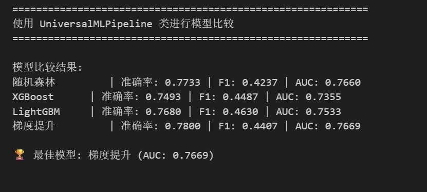
# 3. 一键比较所有模型
print("=" * 60)
print("使用 UniversalMLPipeline 类进行模型比较")
print("=" * 60)
results = ml_pipeline.compare_models(X_train, X_test, y_train, y_test, models_to_compare)
# 4. 打印结果
print("\n模型比较结果:")
for name, result in results.items():
print(f"{name:12s} | 准确率: {result['accuracy']:.4f} | F1: {result['f1']:.4f} | AUC: {result['roc_auc']:.4f}")
# 5. 获取最佳模型
best = ml_pipeline.get_best_model('roc_auc')
print(f"\n🏆 最佳模型: {best['model_name']} (AUC: {best['roc_auc']:.4f})")