Matlab的主成分分析pca函数的使用方法

主成分分析(Principal Component Analysis, PCA)是最常用的无监督降维方法。它的工作原理可以从很多教科书中找到，工作流程如下：

其中，m表示样本个数，X表示样本矩阵（大小为m*d，即每行对应一个样本），最后得到投影矩阵W（大小为d*d'），可以将样本从d维降到d'维。

最近想使PCA处理一下数据，于是乎研究了一下Matlab中内置的pca函数。使用之前，当然是使用"help pca"看一下函数的帮助信息。

pca Principal Component Analysis (pca) on raw data.

COEFF = pca(X) returns the principal component coefficients for the N

by P data matrix X. Rows of X correspond to observations and columns to

variables. Each column of COEFF contains coefficients for one principal

component. The columns are in descending order in terms of component

variance (LATENT). pca, by default, centers the data and uses the

singular value decomposition algorithm. For the non-default options,

use the name/value pair arguments.

$COEFF, SCORE$ = pca(X) returns the principal component score, which is

the representation of X in the principal component space. Rows of SCORE

correspond to observations, columns to components. The centered data

can be reconstructed by SCORE*COEFF'.

$COEFF, SCORE, LATENT$ = pca(X) returns the principal component

variances, i.e., the eigenvalues of the covariance matrix of X, in

LATENT.

$COEFF, SCORE, LATENT, TSQUARED$ = pca(X) returns Hotelling's T-squared

statistic for each observation in X. pca uses all principal components

to compute the TSQUARED (computes in the full space) even when fewer

components are requested (see the 'NumComponents' option below). For

TSQUARED in the reduced space, use MAHAL(SCORE,SCORE).

$COEFF, SCORE, LATENT, TSQUARED, EXPLAINED$ = pca(X) returns a vector

containing the percentage of the total variance explained by each

principal component.

$COEFF, SCORE, LATENT, TSQUARED, EXPLAINED, MU$ = pca(X) returns the

estimated mean.

$...$ = pca(..., 'PARAM1',val1, 'PARAM2',val2, ...) specifies optional

parameter name/value pairs to control the computation and handling of

special data types. Parameters are:

'Algorithm' - Algorithm that pca uses to perform the principal

component analysis. Choices are:

'svd' - Singular Value Decomposition of X (the default).

'eig' - Eigenvalue Decomposition of the covariance matrix. It

is faster than SVD when N is greater than P, but less

accurate because the condition number of the covariance

is the square of the condition number of X.

'als' - Alternating Least Squares (ALS) algorithm which finds

the best rank-K approximation by factoring a X into a

N-by-K left factor matrix and a P-by-K right factor

matrix, where K is the number of principal components.

The factorization uses an iterative method starting with

random initial values. ALS algorithm is designed to

better handle missing values. It deals with missing

values without listwise deletion (see {'Rows',

'complete'}).

'Centered' - Indicator for centering the columns of X. Choices are:

true - The default. pca centers X by subtracting off column

means before computing SVD or EIG. If X contains NaN

missing values, NANMEAN is used to find the mean with

any data available.

false - pca does not center the data. In this case, the original

data X can be reconstructed by X = SCORE*COEFF'.

'Economy' - Indicator for economy size output, when D the degrees of

freedom is smaller than P. D, is equal to M-1, if data

is centered and M otherwise. M is the number of rows

without any NaNs if you use 'Rows', 'complete'; or the

number of rows without any NaNs in the column pair that

has the maximum number of rows without NaNs if you use

'Rows', 'pairwise'. When D < P, SCORE(:,D+1:P) and

LATENT(D+1:P) are necessarily zero, and the columns of

COEFF(:,D+1:P) define directions that are orthogonal to

X. Choices are:

true - This is the default. pca returns only the first D

elements of LATENT and the corresponding columns of

COEFF and SCORE. This can be significantly faster when P

is much larger than D. NOTE: pca always returns economy

size outputs if 'als' algorithm is specifed.

false - pca returns all elements of LATENT. Columns of COEFF and

SCORE corresponding to zero elements in LATENT are

zeros.

'NumComponents' - The number of components desired, specified as a

scalar integer K satisfying 0 < K <= P. When specified,

pca returns the first K columns of COEFF and SCORE.

'Rows' - Action to take when the data matrix X contains NaN

values. If 'Algorithm' option is set to 'als, this

option is ignored as ALS algorithm deals with missing

values without removing them. Choices are:

'complete' - The default action. Observations with NaN values

are removed before calculation. Rows of NaNs are

inserted back into SCORE at the corresponding

location.

'pairwise' - If specified, pca switches 'Algorithm' to 'eig'.

This option only applies when 'eig' method is used.

The (I,J) element of the covariance matrix is

computed using rows with no NaN values in columns I

or J of X. Please note that the resulting covariance

matrix may not be positive definite. In that case,

pca terminates with an error message.

'all' - X is expected to have no missing values. All data

are used, and execution will be terminated if NaN is

found.

'Weights' - Observation weights, a vector of length N containing all

positive elements.

'VariableWeights' - Variable weights. Choices are:

a vector of length P containing all positive elements.
the string 'variance'. The variable weights are the inverse of

sample variance. If 'Centered' is set true at the same time,

the data matrix X is centered and standardized. In this case,

pca returns the principal components based on the correlation

matrix.

The following parameter name/value pairs specify additional options

when alternating least squares ('als') algorithm is used.

'Coeff0' - Initial value for COEFF, a P-by-K matrix. The default is

a random matrix.

'Score0' - Initial value for SCORE, a N-by-K matrix. The default is

a matrix of random values.

'Options' - An options structure as created by the STATSET function.

pca uses the following fields:

'Display' - Level of display output. Choices are 'off' (the

default), 'final', and 'iter'.

'MaxIter' - Maximum number of steps allowed. The default is

Unlike in optimization settings, reaching

MaxIter is regarded as convergence.

'TolFun' - Positive number giving the termination tolerance for

the cost function. The default is 1e-6.

'TolX' - Positive number giving the convergence threshold

for relative change in the elements of L and R. The

default is 1e-6.

Example:

load hald;

$coeff, score, latent, tsquared, explained$ = pca(ingredients);

See also ppca, pcacov, pcares, biplot, barttest, canoncorr, factoran,

rotatefactors.

我并不关心输入参数，都使用默认设置即可。对于输出参数，可以看到共有六个：

$COEFF, SCORE, LATENT, TSQUARED, EXPLAINED, MU$ = pca(X)

这些输出参数都是什么意思呢？哪个是投影矩阵W？哪个是降维后的样本矩阵呢？我们来简单写个程序看一下。

Matlab 复制代码

X=rand(1000,50);
[COEFF, SCORE, LATENT, TSQUARED, EXPLAINED, MU] = pca(X);

以上是随机生成了一个包含1000个样本（即m=1000）、特征维度为50（即d=50）的样本矩阵X，然后直接调用pca函数对其进行处理。

看一下帮助信息，我们比较感兴趣包括前三个输出参数（COEFF, SCORE, LATENT）和最后一个输出参数（MU）。

首先，MU的含义是最清晰的，它就是PCA第1步中心化时的均值，我们可以做如下验证：

Matlab 复制代码

mean(X)-MU

可以发现这个向量的值都等于0，也可以做如下验证：

Matlab 复制代码

X_mean = X-repmat(MU,1000,1);
mean(X_mean)

也可以发现mean(X_mean)向量的值都等于0。

那么哪个是投影矩阵呢？

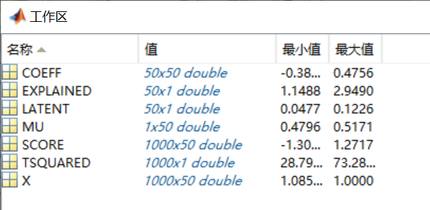
看一下各变量的大小，可以看到COEFF是50*50的，SCORE是1000*50的，因此COEFF应该是投影矩阵W，SCORE则对应投影后的样本矩阵（这里d'仍保留了50维，实际使用时，如果d'小于50，只需取SCORE的前d'列即可，投影矩阵也对应COEFF前d'列）。我们可以做如下验证：

Matlab 复制代码

norm(X_mean*COEFF-SCORE,'fro')

可以发现这个结果等于0，因此结论成立。注意这里使用的是中心化后的X_mean矩阵。

还有一个关键的参数就是PCA算法中做特征值分解得到的特征值是多少？因为在PCA使用时，我们还经常使用特征值所占比例来确定降维后保留的维度数。看帮助信息猜测可能是LATENT，因为帮助信息中解释说是LATENT对应the eigenvalues of the covariance matrix of X。为了验证一下这个结果，我们按照PCA的工作原理来自己实现一下：

Matlab 复制代码

[V,D] = eig(X_mean'*X_mean); 
D_vec = diag(D);
[sort_val, sort_idx] = sort(D_vec,'descend');

我们发现sort_val与LATENT并不相同，而且差异还比较大。

想弄清楚为什么，只能使用"edit pca"来看一下pca函数的具体实现了。细究之后可以发现，pca实际上是使用如下几行代码实现的特征值分解，并得到各输出参数的：

Matlab 复制代码

[U,sigma,coeff] = svd(X_mean,'econ');
sigma = diag(sigma);
score =  bsxfun(@times,U,sigma');
latent = sigma.^2./DOF;

这里的DOF在本例中是常数999。其中，latent就是pca输出的LATENT，score就是输出的SCORE。我们可以发现，latent是SVD分解得到的sigma平方后除以常数DOF得到的。根据SVD的原理，可以猜测sigma.^2对应的就是我们使用eig做特征值分解得到的sort_val，可以做如下验证：

Matlab 复制代码

norm(sort_val- sigma.^2)

可以发现这个结果等于0，因此结论成立。至于说为什么要除以DOF，就不得而知了，但由于DOF是一个常数，所以在计算特征值所占比例时它并没有任何影响，所以可以放心地将pca输出的LATENT当作特征值使用。

到这里，其实该验证的也验证完了，但最后想看一下自己实现的PCA的投影矩阵与pca函数输出的投影矩阵COEFF是否有区别，于是对比了一下：

Matlab 复制代码

V_descend = V(:,sort_idx);
dif_coeff = COEFF-V_descend;

以上是先将V的列按特征值大小降序排列，然后再与COEFF作对比。但发现得到的结果dif_coeff并不是全零矩阵，而是有些列为0，有些列不为0。这就很奇怪了，对比了一下COEFF和V_descend两个投影矩阵，可以发现它们有些列相同，有些列符号相反（也就是多了一些负号），仅此而已，但具体原因并不清楚。

实际上，投影矩阵的某一列差上一个负号，影响的只是最终降维得到的样本矩阵对应的那一列特征多一个负号而已，这在使用时并没有什么影响（比如把X全部变成-X，去学习一个线性分类器w，若将使用X学得的分类器参数记为w，则-X学得的分类器就是-w，效果上是等价的；若X的部分列多一个负号，则就是向量w中对应的元素多一个负号）。

到此，基本所有问题都弄清楚了，我们来总结一下：

对于一个m*d的样本矩阵X来说：

$COEFF, SCORE, LATENT, TSQUARED, EXPLAINED, MU$ = pca(X);

MU是一个1*d的向量，保存的是用于中心化预处理的各特征均值；

COEFF是投影矩阵W，大小为d*d，需要保留d'维则只使用COEFF的前d'列；

SCORE是降维后的样本矩阵，大小为m*d，需要保留d'维则只使用COEFF的前d'列，其中SCORE=X*COEFF（注意X要做中心化）；

LATENT是特征值的变体，其值为特征值除以DOF（是一个常数，一般等于m-1）。

唯一的疑问是投影矩阵COEFF的部分列与自己使用特征值分解动手实现的结果相差一个负号，虽然在使用上并没有什么实质影响，但这样做的原因并不明确。

注：以上过程是使用的是Matlab R2014a验证的。