机器学习笔记

引入

机器学习是一门多学科交叉专业，涉及概率论、统计学、逼近论、凸分析、算法复杂度理论等多门学科，专门研究计算机怎样模拟或实现人类的学习行为，以获取新的知识或技能，重新组织已有的知识结构使之不断改善自身的性能。它是人工智能核心，是使计算机具有智能的根本途径。

问题概述

以线性回归为例

找到一个最能拟合该数据的一个平面

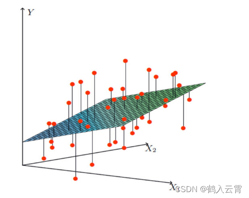
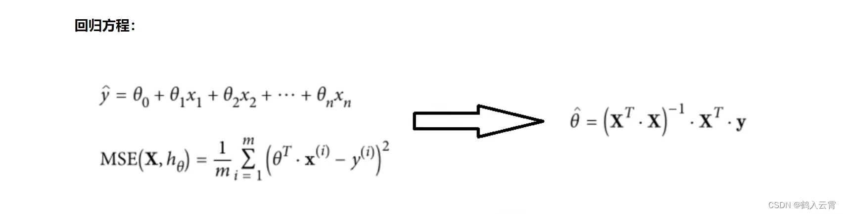
拟合的平面：

：偏置项（微调）

... ：权重（核心）

构造一列x0得到整合后的公式：

已知：

去求解：

线性回归

介绍：

线性回归是机器学习中最基础的回归算法之一，它是一种用于预测一个或多个自变量与因变量之间线性关系的方法。它的目标是建立一个线性方程，该方程可以根据输入变量的值来预测输出变量的值。

线性回归是利用数理统计中回归分析，来确定两种或两种以上变量间相互依赖的定量关系的一种统计分析方法，运用十分广泛。其表达形式为y = w'x+e，e为误差服从均值为0的正态分布。回归分析中，只包括一个自变量和一个因变量，且二者的关系可用一条直线近似表示，这种回归分析称为一元线性回归分析。如果回归分析中包括两个或两个以上的自变量，且因变量和自变量之间是线性关系，则称为多元线性回归分析。

线性回归在机器学习算法中具备基础地位。它可以帮助人们更好地理解数据的性质和关系，为后续更复杂的机器学习算法提供基础。

误差项定义：

误差项是指观测值与预测值之间的差异，是不能由X和Y的线性关系所解释的Y的变异性。

真实值和预测值之间存在的差异（用表示误差）

对于每个样本：（1）

期待的误差项为越小越好

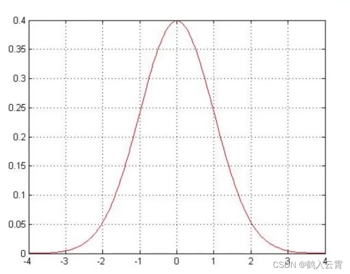
是独立并且具有相同的分布，并且服从均值为0方差为的高斯分布

独立：张三和李四一起来贷款，他俩没关系

同分布：他俩来的是我们假定的这家银行

高斯分布：银行可能会多给，也可能会少给，但是绝大多数情况下这个浮动不会太大，极少情况下浮动会比较大，符合正常情况

参数求解：

由于误差服从高斯分布：（2）

将（1）式代入（2）式：

对数似然（Log-Likelihood）是统计学中一种常用的方法，用于估计模型参数。在概率统计中，似然函数表示给定观测数据，关于模型参数的概率分布。对数似然则是似然函数取对数后的结果。

似然函数：

解释为什么用：

1.通过大量数据找到最合适的一个参数

2.在独立同分布的条件下，联合密度等于各个变量的边缘密度的乘积

对数似然：

解释：乘法难解，加法就容易了，对数厘米乘法可以转化成加法

展开化简：

似然函数计算的是预测值和真实值的可能性，所以似然函数越大越好

目标：让似然函数（对数变换后也一样）越大越好 --> 越小它才能越大

（最小二乘法）

目标函数：

这里的x,y,theta都为矩阵，矩阵的平方等于转置乘它本身

求偏导：过程略

偏导等于0时，求出的极值点：

梯度下降：

沿着梯度的反方向走

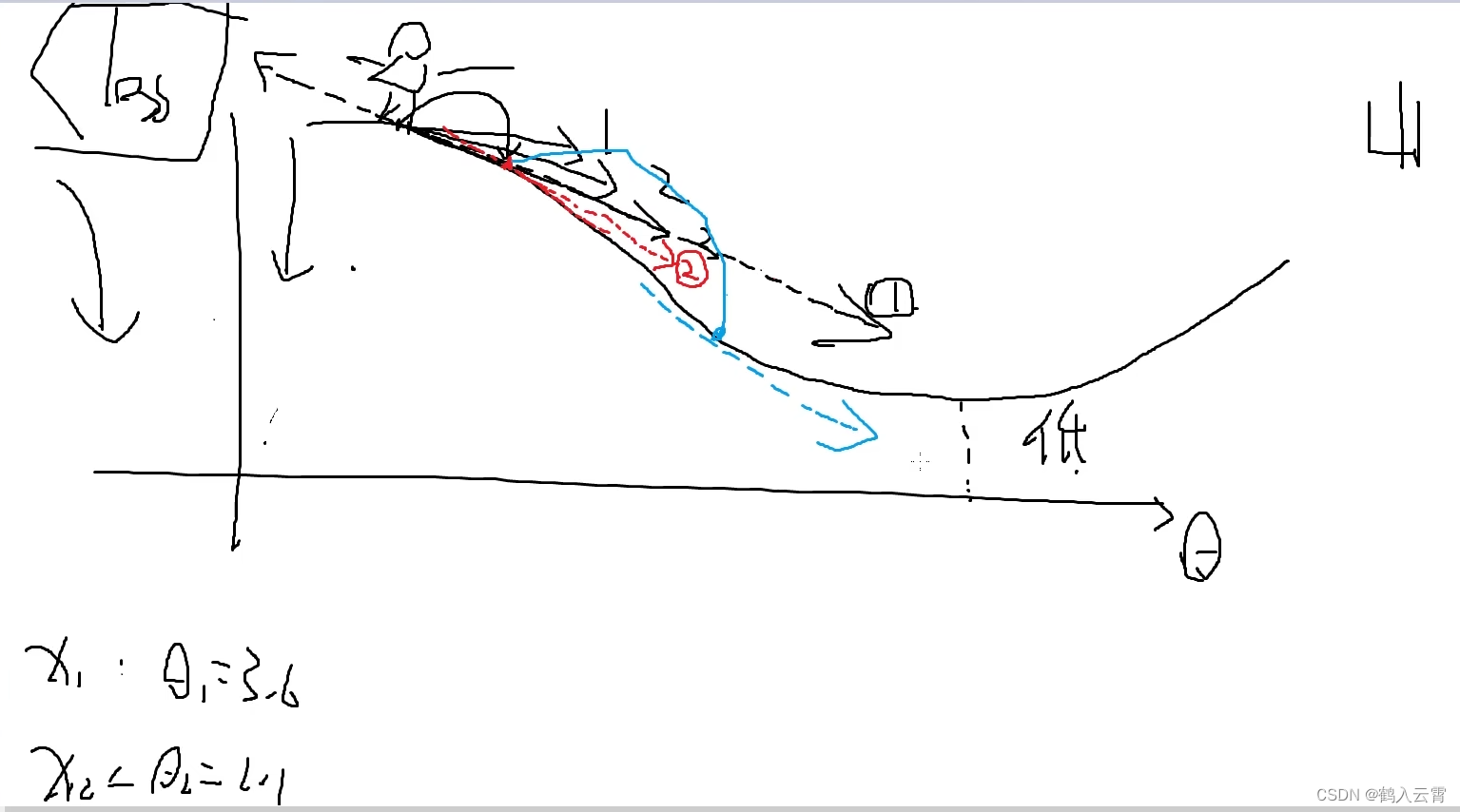
机器学习的常规套路：交给机器一堆数据，然后告诉它什么样的学习方式是对的（目标函数），然后让它朝着这个方向去做

如何优化：静悄悄的一步步完成迭代（每次优化一点点，累积起来就是个大成绩了）

目标函数：

批量梯度下降：

矩阵：

这是梯度下降法最原始的形式。在更新每一参数时都使用所有的样本来进行更新。由于是最小化风险函数，所以按照每个参数的梯度负方向来更新每个参数。其优点是全局最优解，易于并行实现，缺点是当样本数目很大时，训练过程会很慢。

容易得到最优解，但每次都要考虑所有样本，速度很慢

随机梯度下降：

每次迭代只使用一个样本来进行参数更新，可以加速训练过程。

每次找一个样本，迭代速度快，但不一定每次都朝着收敛的方向

小批度梯度下降：

介于批量梯度下降和随机梯度下降之间，通过将数据集分成若干小样本进行模型训练，可以在保证一定训练速度的同时，尽可能地提高模型训练的准确性。

每次更新选择一小部分数据来算，实用！

这三种方法都是用来优化模型的参数，使其能够更好地拟合数据、降低预测误差。在实际应用中，可以根据具体问题和数据集的特点选择合适的方法。

学习率（步长）：

学习率是在所有的梯度下降法中都存在的一个超参数。它控制着模型学习的速度，即在多大程度上调整网络的权重。具体而言，它影响的是每次参数更新的步长。学习率设置得过大，可能会导致模型在最优解附近震荡而无法收敛；学习率设置得过小，则可能会导致模型收敛速度过慢。因此，合适的学习率设置对于模型的训练效果至关重要。

线性回归整体模块实现

linear_regression.py 线性回归算法模型

python 复制代码

# 导入矩阵运算库
import numpy as np 
# 导入数据预处理方法
from utils.features.prepare_for_training import prepare_for_training


# 计算的东西很多可以定义一个类
class LinearRegression:

    def __init__(self, data, labels, polynomial_degree=0, sinusoid_degree=0, normalize_data=True):  # 初始化函数里传入要用的值
        """
        1.对数据进行预处理操作
        2.先得到所有的特征个数
        3.初始化参数矩阵
        """
        # 进行数据预处理，然后将结果保存到新变量中
        # data_processed 预处理完后的数据，相当于标准化后的结果
        # features_mean 平均值
        # features_deviation 标准差
        (data_processed, features_mean, features_deviation) = prepare_for_training(data, polynomial_degree, sinusoid_degree, normalize_data)
        # 将data进行更新
        self.data = data_processed
        # 标签没变，还是之前的标签
        self.labels = labels
        # 下面的值都为初始化函数传入值
        self.features_deviation = features_deviation
        self.polynomial_degree = polynomial_degree
        self.sinusoid_degree = sinusoid_degree
        self.normalize_data = normalize_data
        # 构建theta参数，theta个数跟特征的个数相等
        # 所以先计算出特征数量，.shape之后为行和列
        num_features = self.data.shape[1]
        """
        初始的 theta 设定为全零矩阵是为了在开始时没有任何预判或偏见。这也是许多机器学习算法（如线性回归、逻辑回归等）的默认设置。
        通过训练过程,将更新 theta 以最小化预测值与实际值之间的差异。这样，theta 就会成为模型的一部分，用于将输入特性转换为预测结果。
        注意：这里的 theta 是一个列向量，而不是一个矩阵
        """
        self.theta = np.zeros((num_features, 1))

    def train(self, alpha, num_iterations=500):
        """
        alpha 学习率
        num_iterations  迭代次数
        """
        cost_history = self.gradient_descent(alpha, num_iterations)
        return self.theta, cost_history

    def gradient_descent(self, alpha, num_iterations):
        """
        这里要进行参数更新，梯度计算
        """
        # 用于可视化展示
        cost_history = []
        for _ in range(num_iterations):       
            self.gradient_step(alpha)
            cost_history.append(self.cost_function(self.data, self.labels))
        return cost_history

    def gradient_step(self, alpha):
        """
        数学公式
        梯度下降参数更新计算方法，注意是矩阵运算
        """
        # 样本个数 [0]所有行，[1]所有列
        num_examples = self.data.shape[0]
        # 预测值 = 真实值（当前数据） * 当前参数
        prediction = LinearRegression.hypothesis(self.data, self.theta)
        # 误差 = 预测值 - 真实值
        delta = prediction - self.labels
        theta = self.theta
        # 点积运算要求 delta 和 self.data 的行数相匹配，delta.T 对delta进行转置（行和列互换）
        theta = theta - alpha * (1/num_examples) * (np.dot(delta.T, self.data)).T
        # 更新theta
        self.theta = theta
    
    def cost_function(self, data, labels):
        """
        计算损失
        当前损失 = （数据 * 当前参数参数值）与 label 进行比较   
        """   
        # 公平起见，用于求平均，防止样本多的多算
        num_examples = data.shape[0]  
        delta = LinearRegression.hypothesis(self.data, self.theta) - labels
        # / num_examples: 损失值是用来评判模型好坏的，应该与样本个数无关
        # 下面乘（1/2）只是为了求导的计算过程更加方便，理解为方便计算就好，没有也是可以的！
        cost = (1 / 2) * np.dot(delta.T, delta) / num_examples
        # print(cost.shape)
        # print(cost)
        """
        虽然cost是一个矩阵，但他表示的就是(y'-y)²+...+ (y'-y)²
        """
        return cost[0][0]

    @staticmethod  # 该函数里没有用到self，加入这句可以直接调用类中的方法，无需再实例化对象
    def hypothesis(data, theta):
        """
        预测函数，计算预测值
        """
        predictions = np.dot(data, theta)
        return predictions
        

    def get_cost(self, data, labels):
        # 经过处理了的数据
        data_processed = prepare_for_training(data,
                                              self.polynomial_degree,
                                              self.sinusoid_degree,
                                              self.normalize_data)[0]
        return self.cost_function(data_processed, labels)  # 返回损失值

    def predict(self, data):
        """
        用训练的数据模型，预测得到回归值结果
        """
        # 经过处理了的数据
        data_processed = prepare_for_training(data,
                                              self.polynomial_degree,
                                              self.sinusoid_degree,
                                              self.normalize_data)[0]
        predictions = LinearRegression.hypothesis(data_processed, self.theta)
        return predictions  # 返回预测值

补充

损失函数是用于衡量预测值与实际值偏离程度的函数，误差项则通常是指预测值与实际值之间的差值，这个差值可以是绝对差或相对差，误差项是损失函数的一部分，用于计算损失函数的值。
cost_function函数的损失值（均方误差）计算公式为：

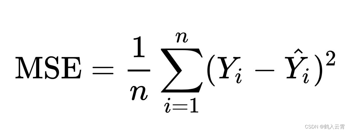
np. dot(,)

对于两个一维向量，会进行点积运算

对于两个二维数组，会进行矩阵乘法

如果是求两个数组的平方，要对其中一个数组进行转置（需要确保两个数组的形状是相同的）

utils.features.normalize.py 标准化

python 复制代码

import numpy as np

def normalize(features):
    # astype：转换数组的数据类型
    features_normalized = np.copy(features).astype(float)

    # 计算均值
    features_mean = np.mean(features, 0)

    # 计算标准差
    features_deviation = np.std(features, 0)

    # 标准化操作
    if features.shape[0] > 1:
        features_normalized -= features_mean
    # 防止除以0 （分母为0）
    features_deviation[features_deviation == 0] = 1
    features_normalized /= features_deviation

    return features_normalized, features_mean, features_deviation

补充

标准化公式：标准化后的数据每列的均值为0，标准差为1。

即：x 减 x轴的均值，y减 y轴的均值

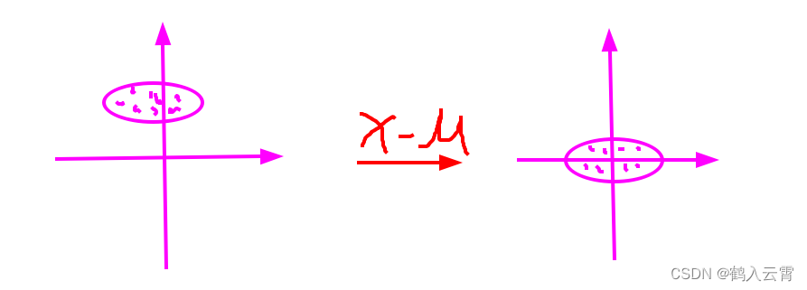
无论几维特征，原数据减去各自的均值，就可以得到一个以原点为中心，对称的数据

utils.features.prepare_for_training.py 数据预处理

python 复制代码

import numpy as np
from .normalize import normalize

def prepare_for_training(data, polynomial_degree=0, sinusoid_degree=0, normalize_data=True):
    # 计算样本总数
    num_examples = data.shape[0]

    data_processed = np.copy(data)

    # 预处理
    features_mean = 0
    features_deviation = 0
    data_normalized = data_processed
    if normalize_data:
        (
            data_normalized,
            features_mean,
            features_deviation
        ) = normalize(data_processed)    # 执行标准化

        data_processed = data_normalized
    
    
    """
    加一列1，为了方便做矩阵运算：
    创建一个全为 1 的列向量，其形状为 (num_examples, 1)。
    使用 hstack 将这个全为 1 的列向量和 data_processed 水平堆叠在一起。
    """
    data_processed = np.hstack((np.ones((num_examples, 1)), data_processed))

    return data_processed, features_mean, features_deviation

UnivariataLinearRegression.py 线性回归应用（单特征）

python 复制代码

import numpy as np
import pandas as pd
import matplotlib.pyplot as plt
from linear_regression import LinearRegression


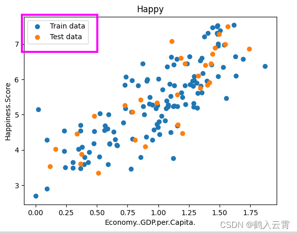
data = pd.read_csv('../data/world-happiness-report-2017.csv')

# 得到训练和测试数据集
train_data = data.sample(frac=0.8)  # sample：随机选取若干行
test_data = data.drop(train_data.index)  # 将训练数据删除即为测试数据

# 数据和标签定义
input_param_name = "Economy..GDP.per.Capita."
output_param_name = "Happiness.Score"

# .values属性将pandas DataFrame转换为numpy数组
x_train = train_data[[input_param_name]].values
y_train = train_data[[output_param_name]].values

x_test = test_data[[input_param_name]].values
y_test = test_data[[output_param_name]].values

# 定义训练参数
num_iterations = 500  
learning_rate = 0.01  

linear_regression = LinearRegression(x_train, y_train)
# 执行训练
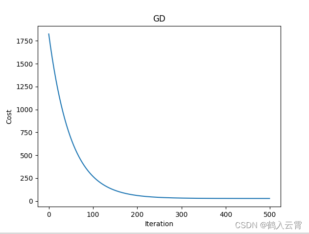
(theta, cost_history) = linear_regression.train(learning_rate, num_iterations)  

print('开始时的损失', cost_history[0])
print('训练后的损失', cost_history[-1])  # 最后一个

plt.plot(range(num_iterations), cost_history)
plt.xlabel('Iteration')
plt.ylabel('Cost')
plt.title('GD')
plt.show()

# 测试
predications_num = 100
"""
从训练数据的最小值到最大值之间生成predications_num个等间隔的值
使用.reshape(predications_num, 1)将这些值重塑为一个形状为(predications_num, 1)的二维数组。这样做的目的是为了满足线性回归模型predict()方法所需的输入格式
x_predications:筛选出要预测的数据
y_predications:得到预测后的数据
"""
x_predications = np.linspace(x_train.min(), x_train.max(), predications_num).reshape(predications_num, 1)
y_predications = linear_regression.predict(x_predications)

plt.scatter(x_train, y_train, label="Train data")
plt.scatter(x_test, y_test, label="Test data")
plt.plot(x_predications, y_predications, 'r', label="预测值")
plt.xlabel(input_param_name)
plt.ylabel(output_param_name)
plt.title("Happy test")
plt.legend()
plt.show()

补充

pandas 库中的 .sample()：从数据框（DataFrame）中随机选取一定比例的行

data.sample(frac=0.8) 会返回一个新的数据框，其中包含原数据框中80%的行。这些行的选取是随机的，可以有效地用于训练模型，而剩下的20%的数据则作为测试数据集，用于评估模型的性能。

pandas库中的 .drop()：将train_data中的索引对应的行从原始数据data中删除，留下的部分即为test_data。

3. plt.scatter 是 Matplotlib 库中的一个函数，用于创建散点图。散点图是一种在二维平面上绘制一系列点的图表，通常用于显示两个变量之间的关系

x 和 y 是数组，表示数据点的 x 坐标和 y 坐标。
**kwargs 是可选参数，用于设置散点图的外观，例如颜色、大小、形状等。

4. plt.legend() 是 matplotlib 库中的一个函数，用于在图表中添加图例

5.plt.plot() 创建一个二维折线图

6. np.linspace()函数来创建一个等间隔的数值数组

start：数值范围的起始值。
stop：数值范围的结束值。
num：需要生成的数值数量。

MultivariateLinearRegression.py 线性回归应用（多特征）

python 复制代码

import numpy as np
import pandas as pd
import matplotlib.pyplot as plt
import plotly  # 交互式界面展示
import plotly.graph_objs as go
# plotly.offline.init_notebook_mode() ipython or notebook used
from linear_regression import LinearRegression

data = pd.read_csv('../data/world-happiness-report-2017.csv')
train_data = data.sample(frac=0.8)  
test_data = data.drop(train_data.index)  

# 多了一个input_param_name_2特征
input_param_name_1 = "Economy..GDP.per.Capita."
input_param_name_2 = "Freedom"
output_param_name = "Happiness.Score"

x_train = train_data[[input_param_name_1, input_param_name_2]].values
y_train = train_data[[output_param_name]].values

x_test = test_data[[input_param_name_1, input_param_name_2]].values
y_test = test_data[[output_param_name]].values

# 训练集
plot_training_trace = go.Scatter3d(
    x=x_train[:, 0].flatten(),
    y=x_train[:, 1].flatten(),
    z=y_train.flatten(),
    name="Training Set",
    mode="markers",
    marker={
        'size': 10,
        'opacity': 1,
        'line': {
            'color': 'rgb(255, 255, 255)',
            'width': 1
        }
    }
)

# 测试集
plot_test_trace = go.Scatter3d(
    x=x_test[:, 0].flatten(),
    y=x_test[:, 1].flatten(),
    z=y_test.flatten(),
    name="Test Set",
    mode="markers",
    marker={
        'size': 10,
        'opacity': 1,
        'line': {
            'color': 'rgb(255, 255, 255)',
            'width': 1
        }
    }
)

# 布局
plot_layout = go.Layout(
    title='Date Sets',
    scene={
        'xaxis': {'title': input_param_name_1},
        'yaxis': {'title': input_param_name_2},
        'zaxis': {'title': output_param_name}
    },
    margin={'l': 0, 'r': 0, 'b': 0, 't': 0}
)

# 指定轨迹
plot_data = [plot_training_trace, plot_test_trace]
# 绘图
plot_figure = go.Figure(data=plot_data, layout=plot_layout)
plotly.offline.plot(plot_figure)  

num_iterations = 500
learning_rate = 0.01  # 学习率
polynomial_degree = 0
sinusoid_degree = 0

linear_regression = LinearRegression(x_train, y_train, polynomial_degree, sinusoid_degree)

(theta, cost_history) = linear_regression.train(
    learning_rate,
    num_iterations
)
print('开始损失', cost_history[0])
print('结束损失', cost_history[-1])
plt.plot(range(num_iterations), cost_history)
plt.xlabel('Iterations')
plt.ylabel('Cost')
plt.title('Gradient Descent Progress')
plt.show()

predictions_num = 10

x_min = x_train[:, 0].min()
x_max = x_train[:, 0].max()

y_min = x_train[:, 1].min()
y_max = x_train[:, 1].max()

x_axis = np.linspace(x_min, x_max, predictions_num)
y_axis = np.linspace(y_min, y_max, predictions_num)

x_predictions = np.zeros((predictions_num * predictions_num, 1))
y_predictions = np.zeros((predictions_num * predictions_num, 1))

x_y_index = 0
for x_index, x_value in enumerate(x_axis):
    for y_index, y_value in enumerate(y_axis):
        x_predictions[x_y_index] = x_value
        y_predictions[x_y_index] = y_value
        x_y_index += 1
z_predictions = linear_regression.predict(np.hstack((x_predictions, y_predictions)))

plot_predictions_trace = go.Scatter3d(
    x=x_predictions.flatten(),
    y=y_predictions.flatten(),
    z=z_predictions.flatten(),
    name='Prediction Plane',
    marker={
        'size': 1,
    },
    opacity=0.8,
    surfaceaxis=2
)

plot_data = [plot_training_trace, plot_test_trace, plot_predictions_trace]
plot_figure = go.Figure(data=plot_data, layout=plot_layout)
plotly.offline.plot(plot_figure)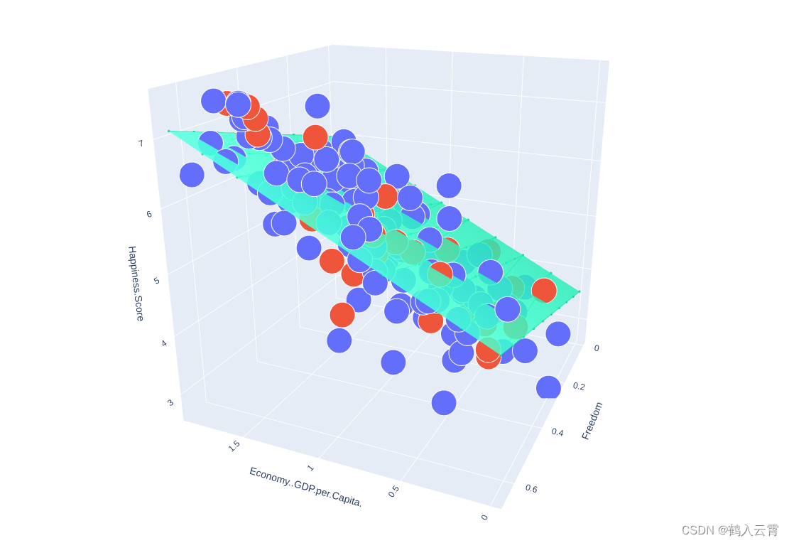

补充

plotly 的模板及使用方法：Plotly Python Graphing Library
flatten()函数将一个多维数组转换为一个一维数组
plotly.offline.plot(plot_figure) 弹出浏览器网页展示， plotly.offline.iplot(plot_figure) 在notebook中嵌入展示
go.Scatter3d() 用于创建三维散点图
上述代码中的x表示第一个特征，y表示第二个特征，z表示标签即幸福指数

非线性模型实现

模型会比较复杂，非常容易过拟合

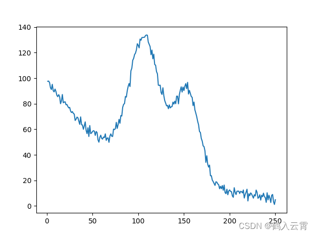不规则曲线的数据

得到非线性模型的做法和前面其实是一样的，只不过这里需要（可以）加入特征变换：

进行特征变换，使特征更丰富

特征变换可以帮助简化模型，提高模型的准确率和泛化能力

特征变换可以有效降低损失值

prepare_for_training.py

需要加入特征变换（sinusoid、polynomial）

python 复制代码

from .generate_sinusoids import generate_sinusoids
from .generate_polynomials import generate_polynomials


import numpy as np
from .normalize import normalize
from .generate_sinusoids import generate_sinusoids
from .generate_polynomials import generate_polynomials

"""数据预处理"""


def prepare_for_training(data, polynomial_degree=0, sinusoid_degree=0, normalize_data=True):
    # 计算样本总数
    num_examples = data.shape[0]

    data_processed = np.copy(data)

    # 预处理
    features_mean = 0
    features_deviation = 0
    data_normalized = data_processed
    if normalize_data:
        (
            data_normalized,
            features_mean,
            features_deviation
        ) = normalize(data_processed)  # 执行标准化

        data_processed = data_normalized

    # 特征变换sinusoid
    if sinusoid_degree > 0:
        sinusoids = generate_sinusoids(data_normalized, sinusoid_degree)
        data_processed = np.concatenate((data_processed, sinusoids), axis=1)

    # 特征变换polynomial
    if polynomial_degree > 0:
        polynomials = generate_polynomials(data_normalized, polynomial_degree, normalize_data)
        data_processed = np.concatenate((data_processed, polynomials), axis=1)

    # 加一列1
    data_processed = np.hstack((np.ones((num_examples, 1)), data_processed))

    return data_processed, features_mean, features_deviation

generate_polynomials.py

python 复制代码

"""Add polynomial features to the features set 将多项式特征添加到特征集"""

import numpy as np
from .normalize import normalize


def generate_polynomials(dataset, polynomial_degree, normalize_data=False):
    """变换方法：
    x1, x2, x1^2, x2^2, x1*x2, x1*x2^2, etc.

    :param dataset: dataset that we want to generate polynomials for.
    :param polynomial_degree: the max power of new features.
    :param normalize_data: flag that indicates whether polynomials need to normalized or not.
    """
    # Split features on two halves.
    features_split = np.array_split(dataset, 2, axis=1)
    dataset_1 = features_split[0]
    dataset_2 = features_split[1]

    # Extract sets parameters.
    (num_examples_1, num_features_1) = dataset_1.shape
    (num_examples_2, num_features_2) = dataset_2.shape

    if num_examples_1 != num_examples_2:
        raise ValueError('Can not generate polynomials for two  sets with different number of rows')

    if num_features_1 == 0 and num_features_2 == 0:
        raise ValueError('Can not generate polynomials for two sets with no columns')

    # Replace empty set with non-empty one.
    if num_features_1 == 0:
        dataset_1 = dataset_2
    elif num_features_2 == 0:
        dataset_2 = dataset_1

    # Make sure that sets have the same number of features in order to be able to multiply them.
    num_features = num_features_1 if num_features_1 < num_examples_2 else num_features_2
    dataset_1 = dataset_1[:, :num_features]
    dataset_2 = dataset_2[:, :num_features]

    # Create polynomials matrix.
    polynomials = np.empty((num_examples_1, 0))

    # Generate polynomial features of specified degree.
    for i in range(1, polynomial_degree + 1):
        for j in range(i + 1):
            polynomial_feature = (dataset_1 ** (i - j)) * (dataset_2 ** j)
            polynomials = np.concatenate((polynomials, polynomial_feature), axis=1)

    # Normalize polynomials if needed.
    if normalize_data:
        polynomials = normalize(polynomials)[0]

    # Return generated polynomial features.
    return polynomials

generate_sinusoids.py

python 复制代码

import numpy as np

def generate_sinusoids(dataset, sinusoid_degree):
    """
    Returns a new feature array with more features, comprising of
    sin(x).非线性变换
    """
    # Create sinusoids matrix.
    num_examples = dataset.shape[0]
    sinusoids = np.empty((num_examples, 0))

    # Generate sinusoid features of specified degree.
    for degree in range(1, sinusoid_degree + 1):
        sinusoid_features = np.sin(degree * dataset)
        sinusoids = np.concatenate((sinusoids, sinusoid_features), axis=1)

    # Return generated sinusoidal features.
    return sinusoids

补充

上两个代码只要知道它在做什么就好，以后需要用到特征变换的时候直接使用sklearn工具包

Non-linearRegression.py

python 复制代码

import numpy as np
import pandas as pd
import matplotlib.pyplot as plt
from linear_regression import LinearRegression

data = pd.read_csv('../data/non-linear-regression-x-y.csv')

x = data['x'].values.reshape((data.shape[0], 1))
y = data['y'].values.reshape((data.shape[0], 1))

data.head(10)

# visualize the training and test datasets to see the shape of the data
plt.plot(x, y)
plt.show()

# Set up linear regression parameters.
num_iterations = 50000
learning_rate = 0.01
polynomial_degree = 15   # The degree of additional polynomial features.
sinusoid_degree = 15     # The degree of sinusoid parameter multipliers of additional features.
normalize_date = True

# Init linear regression instance.
# linear_regression = LinearRegression(x, y, normalize_date)   # 线性回归
linear_regression = LinearRegression(x, y, polynomial_degree, sinusoid_degree, normalize_date)

# Train linear regression
(theta, cost_history) = linear_regression.train(
    learning_rate,
    num_iterations
)

print('开始损失: {:.2f}'.format(cost_history[0]))
print('结束损失: {:.2f}'.format(cost_history[-1]))

theta_table = pd.DataFrame({'Model Parameters': theta.flatten()})

# Plot gradient descent progress.
plt.plot(range(num_iterations), cost_history)
plt.xlabel('Iterations')
plt.ylabel('Cost')
plt.title('Gradient Descent Progress')
plt.show()

# Get model predictions for the trainint set.
predictions_num = 1000
x_predictions = np.linspace(x.min(), x.max(), predictions_num).reshape(predictions_num,1)
y_predictions = linear_regression.predict(x_predictions)

# Plot training data with predictions.
plt.scatter(x, y, label='Training Dataset')
plt.plot(x_predictions, y_predictions, 'r', label='Prediction')
plt.show()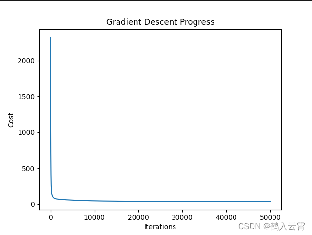

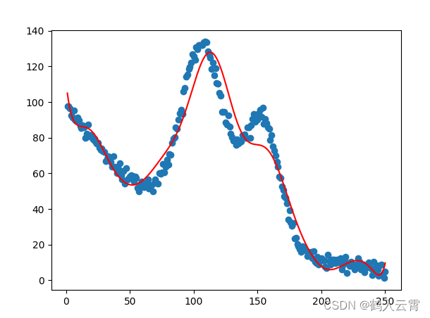蓝：原始数据红：预测数据

线性回归实验分析

此实验重点解释其中每一步流程与实验对比分析

主要内容：

线性回归方程实现
梯度下降效果
对比不同梯度下降策略
建模曲线分析
过拟合与欠拟合
正则化的作用
提前停止策略

线性回归方程实现

参数直接求解法（非机器学习思想）

公式直用实现：

python 复制代码

import matplotlib.pyplot as plt
import numpy as np


plt.rcParams['axes.labelsize'] = 14
plt.rcParams['xtick.labelsize'] = 12
plt.rcParams['ytick.labelsize'] = 12

# 构造数据
X = 2 * np.random.rand(100, 1)
y = 4 + 3 * X + np.random.randn(100, 1)
plt.plot(X, y, 'b.')
plt.xlabel('X_1')
plt.ylabel('y')
plt.axis((0, 2, 0, 15))  # x 轴的值会在 0 到 2 之间变化，而 y 轴的值会在 0 到 15 之间变化。确保了图形在指定的坐标范围内绘制
plt.show()

# 参数直接求解
X_b = np.c_[np.ones((100, 1)), X]  # np.c_ 按列堆叠数组，加一列1

# theta 求解公式
theta_best = np.linalg.inv(X_b.T.dot(X_b)).dot(X_b.T).dot(y)  # np.linalg.inv 求逆
print(theta_best)

# 预测
X_new = np.array([[0], [2]])

X_new_b = np.c_[np.ones((2, 1)), X_new]

# 用预测数据乘最好的那个theta
y_predict = X_new_b.dot(theta_best)

# 画出回归方程
plt.plot(X_new, y_predict, 'r--')
plt.plot(X, y, 'b.')
plt.axis((0, 2, 0, 15))
plt.show()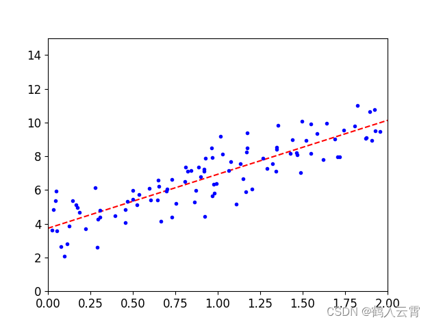

使用sklearn工具包实现（机器学习思想：学习的过程即梯度下降）

python 复制代码

from sklearn.linear_model import LinearRegression
lin_reg = LinearRegression()
lin_reg.fit(X, y)
print(lin_reg.coef_)
print(lin_reg.intercept_)
ypr = lin_reg.predict(X_new)
plt.plot(X_new, ypr, 'r--')
plt.plot(X, y, 'b.')
plt.axis((0, 2, 0, 15))
plt.show()

以上两种方法的theta求解结果，线性回归方程是一致的，sklearn工具包实现更容易些

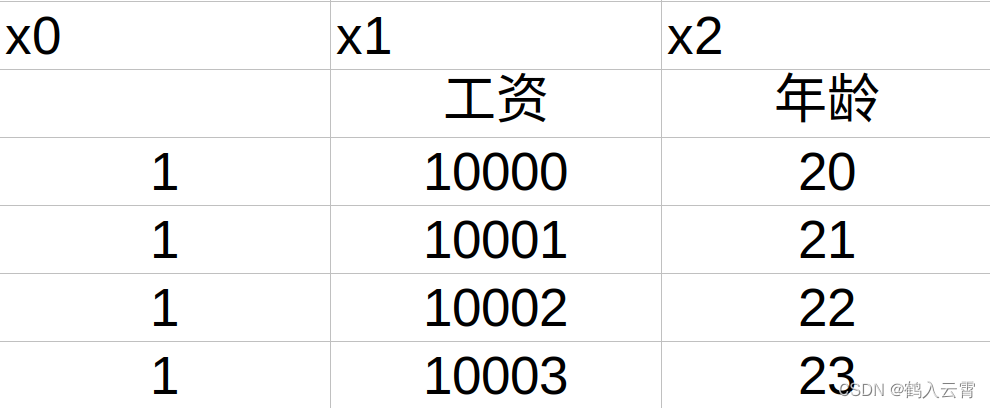
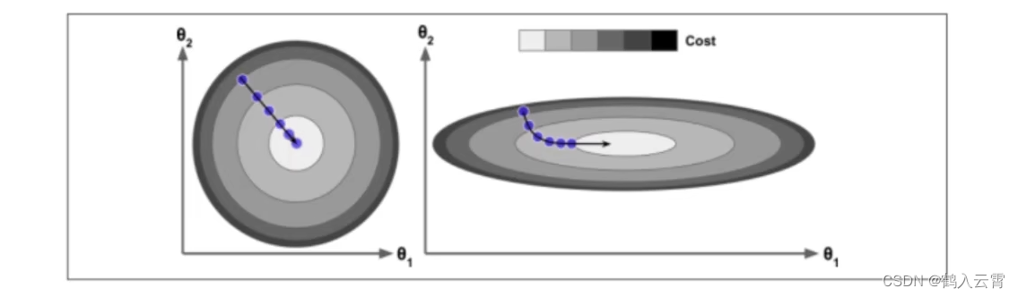
数据预处理对结果的影响

视为年龄，为工资

左：经过数据预处理的，与的取值范围 是相同的，收敛：平稳、快速、一条线

右：未经过数据预处理，与的取值范围 是不同的，导致收敛非常非常慢

由此可以看出数据预处理这一过程是非常有必要的

标准化

数据预处理的一个方法

通过对原始数据进⾏变换把数据变换到均值为0,标准差为1范围内

：前面回归问题概述中有提到

：标准差，数据间的浮动大小

|----|------|
| x1 | x2 |
| 40 | 6000 |
| 30 | 12w |
| 20 | 100w |

x1除一个较小的标准差，x2除一个较大的标准差

除标准差的作用：让数据的取值范围尽可能相同

梯度下降模块

批量梯度下降（BGD）

Batch Gradient Descent

损失函数图像是一条曲线

python 复制代码

import numpy as np

X = 2 * np.random.rand(100, 1)
y = 4 + 3 * X + np.random.randn(100, 1)
X_b = np.c_[np.ones((100, 1)), X]
X_new = np.array([[0], [2]])
X_new_b = np.c_[np.ones((2, 1)), X_new]

eta = 0.1
n_iterations = 1000
m = 100
# 随机初始化
theta = np.random.randn(2, 1)
for _ in range(n_iterations):
    gradients = (2 / m) * X_b.T.dot(X_b.dot(theta) - y)
    theta = theta - eta * gradients

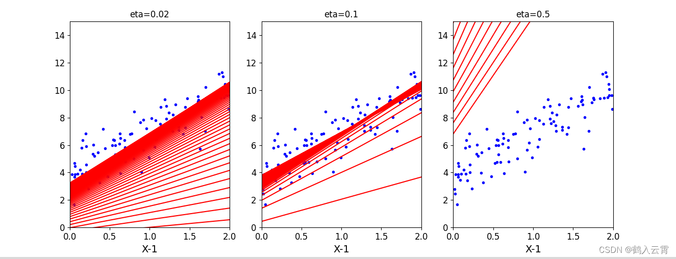
print(X_new_b.dot(theta))

学习率对结果的影响

附代码：

python 复制代码

theta_path_bgd = []
def plot_gradient_descent(theta, eta, theta_path=None):
    m = len(X_b)
    plt.plot(X, y, 'b.')
    n_iterations = 100
    for _ in range(n_iterations):
        y_predict = X_new_b.dot(theta)
        plt.plot(X_new, y_predict, 'r-')
        gradients = 2 / m * X_b.T.dot(X_b.dot(theta) - y)
        theta = theta - eta * gradients
        if theta_path is not None:
            theta_path_bgd.append(theta)
    plt.xlabel('X-1')
    plt.axis((0, 2, 0, 15))
    plt.title('eta={}'.format(eta))

theta = np.random.randn(2, 1)
plt.figure(figsize=(10, 4))
plt.subplot(131)
plot_gradient_descent(theta, eta=0.02)
plt.subplot(132)
plot_gradient_descent(theta, 0.1)
plt.subplot(133)
plot_gradient_descent(theta, 0.5)
plt.show()

随机梯度下降（SGD）

Stochastic Gradient Descent

损失函数图像是抖动的

附代码：

python 复制代码

import numpy as np
import matplotlib.pyplot as plt

plt.rcParams['axes.labelsize'] = 14
plt.rcParams['xtick.labelsize'] = 12
plt.rcParams['ytick.labelsize'] = 12

X = 2 * np.random.rand(100, 1)
y = 4 + 3 * X + np.random.randn(100, 1)
X_b = np.c_[np.ones((100, 1)), X]
X_new = np.array([[0], [2]])
X_new_b = np.c_[np.ones((2, 1)), X_new]

theta_path_sgd = []
m = len(X_b)
n_epochs = 50

t0 = 5
t1 = 50
theta = np.random.randn(2, 1)

# 定义一个学习率调度函数，它返回一个随时间变化的退火学习率。  
def learning_schedule(t):
    return t0 / (t1 + t)


for epoch in range(n_epochs):
    for i in range(m):
        if epoch < 10 and i < 10:
            y_predict = X_new_b.dot(theta)
            plt.plot(X_new, y_predict, 'r-')
        random_index = np.random.randint(m)
        xi = X_b[random_index:random_index+1]
        yi = y[random_index:random_index+1]
        gradients = 2 * xi.T.dot(xi.dot(theta) - yi)
        eta = learning_schedule(n_epochs * m + i)
        theta = theta - eta * gradients
        theta_path_sgd.append(theta)

plt.plot(X, y, 'b.')
plt.axis((0, 2, 0, 15))
plt.show()

小批度梯度下降（MinniBatch）

Mini-batch Gradient Descent

python 复制代码

# 数据同前
theta_path_mgd = []
n_epochs = 50
minibatch = 16
theta = np.random.randn(2, 1)
np.random.seed(0)  # 指定随机种子，使结果相同
t = 0
for epoch in range(n_epochs):
    # 打乱数据
    shuffled_indices = np.random.permutation(m)  # indices -> index 的复数
    X_b_shuffled = X_b[shuffled_indices]
    y_shuffled = y[shuffled_indices]

    for i in range(0, m, minibatch):
        t += 1
        xi = X_b_shuffled[i:i+minibatch]
        yi = y_shuffled[i:i+minibatch]
        gradients = 2 / minibatch * xi.T.dot(xi.dot(theta) - yi)
        eta = learning_schedule(t)
        theta = theta - eta * gradients
        theta_path_mgd.append(theta)

print(theta)

不同策略效果对比

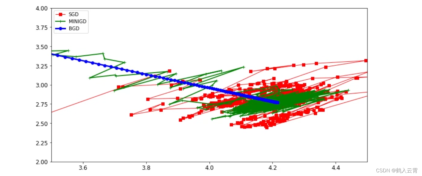
多项式回归

构建数据

python 复制代码

import numpy as np
import matplotlib.pyplot as plt

# 设置字体大小及相关参数
plt.rcParams['axes.labelsize'] = 14
plt.rcParams['xtick.labelsize'] = 12
plt.rcParams['ytick.labelsize'] = 12

# 构建数据
m = 100
X = 6 * np.random.rand(m, 1) - 3
y = 0.5 * X ** 2 + X + np.random.randn(m, 1)

plt.plot(X, y, 'b.')
plt.xlabel('X_1')
plt.ylabel('y')
plt.axis((-3, 3, -5, 10))
plt.show()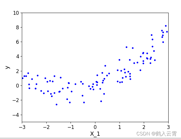

python 复制代码

# 数据变换
from sklearn.preprocessing import PolynomialFeatures
poly_features = PolynomialFeatures(degree=10, include_bias=False)
X_poly = poly_features.fit_transform(X)
print(X[0])
print(X_poly[0])

# 回归方程
from sklearn.linear_model import LinearRegression
lin_reg = LinearRegression()
lin_reg.fit(X_poly, y)
print(lin_reg.coef_)
print(lin_reg.intercept_)

X_new = np.linspace(-3, 3, 100).reshape(100, 1)
X_new_ploy = poly_features.fit_transform(X_new)
y_new = lin_reg.predict(X_new_ploy)
plt.plot(X, y, 'b.')
plt.plot(X_new, y_new, 'r--', label='prediction')
plt.axis((-3, 3, -5, 10))
plt.legend()
plt.show()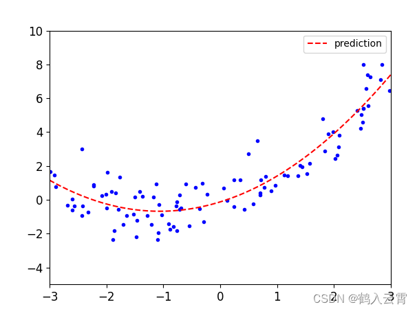

使用sklearn.pipeline对不同degree值的回归方程进行展示

实现代码：

python 复制代码

from sklearn.pipeline import Pipeline
from sklearn.preprocessing import StandardScaler
plt.figure(figsize=(12, 6))
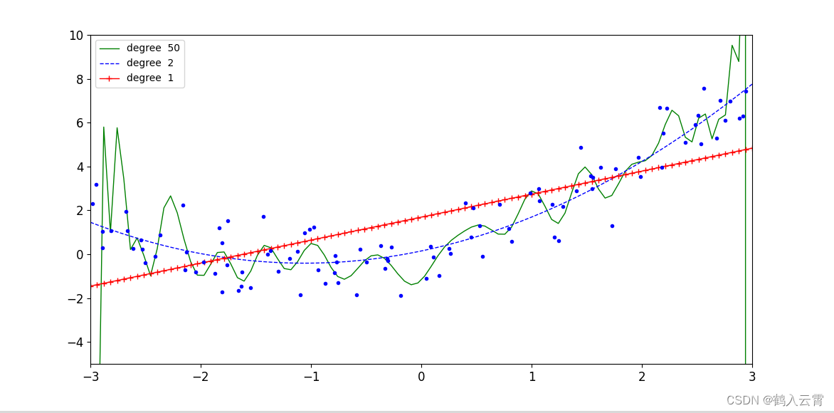
for style, width, degree in (('g-', 1, 50), ('b--', 1, 2), ('r-+', 1, 1)):
    poly_features = PolynomialFeatures(degree=degree, include_bias=False)
    std = StandardScaler()
    lin_reg = LinearRegression()
    polynomial_reg = Pipeline([('poly_features', poly_features),
                               ('StandardScaler', std),
                               ('lin_reg', lin_reg)])
    polynomial_reg.fit(X, y)
    y_new_2 = polynomial_reg.predict(X_new)
    plt.plot(X_new, y_new_2, style, label='degree  '+str(degree), linewidth=width)
plt.plot(X, y, 'b.')
plt.axis((-3, 3, -5, 10))
plt.legend()
plt.show()

当多项式特征的次数（degree）越高，模型更容易发生过拟合

多项式特征的次数越高，意味着模型可以学习到更复杂的函数关系。如果训练数据的质量不高或者数量不够大，那么模型可能会过度拟合训练数据，导致泛化能力下降。

数据样本数量对结果的影响

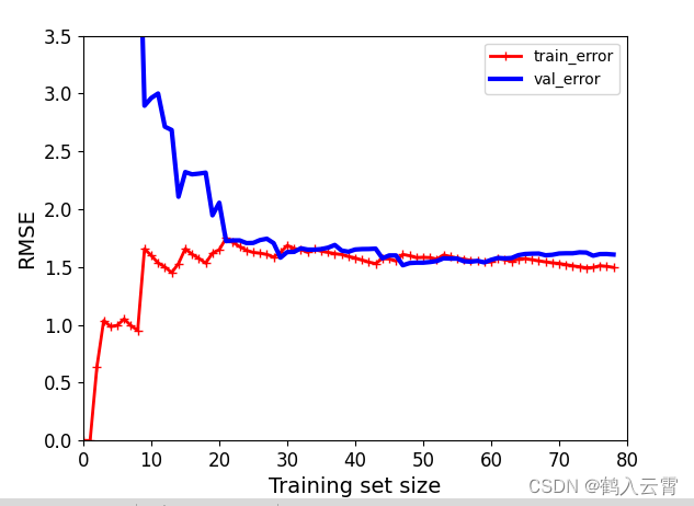
解释：样本数量少的时候，训练集上做的比较好，验证集上做的比较差，

样本数量足够多的时候，考试发挥效果和平时练习效果是比较接近的

实现代码：

python 复制代码

from sklearn.metrics import mean_squared_error
from sklearn.model_selection import train_test_split


def plot_learning_curves(model, X, y):
    X_train, X_val, y_train, y_val = train_test_split(X, y, test_size=0.2, random_state=100)
    train_errors, val_errors = [], []
    for m in range(1, len(X_train)):
        model.fit(X_train[:m], y_train[:m])
        y_train_predict = model.predict(X_train[:m])
        y_val_predict = model.predict(X_val)
        train_errors.append(mean_squared_error(y_train[:m], y_train_predict[:m]))
        val_errors.append(mean_squared_error(y_val, y_val_predict))
    plt.plot(np.sqrt(train_errors), 'r-+', linewidth=2, label='train_error')
    plt.plot(np.sqrt(val_errors), 'b-', linewidth=3, label='val_error')
    plt.xlabel('Training set size')
    plt.ylabel('RMSE')
    plt.legend()


lin_reg = LinearRegression()
plot_learning_curves(lin_reg, X, y)
plt.axis((0, 80, 0, 3.5))
plt.show()

正则化

为了避免过拟合，可以采用一些正则化技术来限制模型的复杂度

对权重参数进行惩罚，让权重参数尽可能平滑一些

岭回归

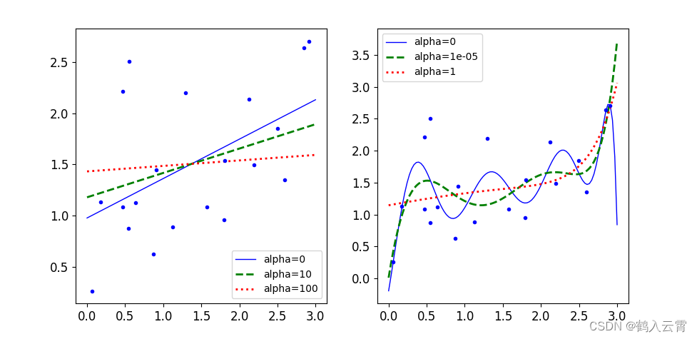
惩罚力度越大，alpha 值越大的时候，得到的决策方程越平稳

python 复制代码

import matplotlib.pyplot as plt
from sklearn.linear_model import Ridge
from sklearn.preprocessing import PolynomialFeatures
from sklearn.pipeline import Pipeline
from sklearn.preprocessing import StandardScaler
import numpy as np

plt.rcParams['axes.labelsize'] = 14
plt.rcParams['xtick.labelsize'] = 12
plt.rcParams['ytick.labelsize'] = 12

np.random.seed(42)
m = 20
X = 3 * np.random.rand(m, 1)
y = 0.5 * X + np.random.randn(m, 1) / 1.5 + 1
X_new = np.linspace(0, 3, 100).reshape(100, 1)


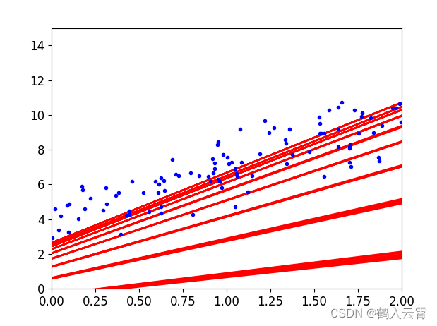
def plot_model(model_class, polynomial, alphas, **model_kargs):
    for alpha, style, in zip(alphas, ('b-', 'g--', 'r:')):
        model = model_class(alpha, **model_kargs)
        if polynomial:
            model = Pipeline([('poly_features', PolynomialFeatures(degree=10, include_bias=False)),
                              ('StandardScaler', StandardScaler()),
                              ('lin_reg', model)])
        model.fit(X, y)
        y_new_regul = model.predict(X_new)
        lw = 2 if alpha > 0 else 1
        plt.plot(X_new, y_new_regul, style, linewidth=lw, label='alpha={}'.format(alpha))
    plt.plot(X, y, 'b.', linewidth=1)
    plt.legend()


plt.figure(figsize=(10, 5))
plt.subplot(121)
plot_model(Ridge, polynomial=False, alphas=(0, 10, 100))
plt.subplot(122)
plot_model(Ridge, polynomial=True, alphas=(0, 10 ** -5, 1))
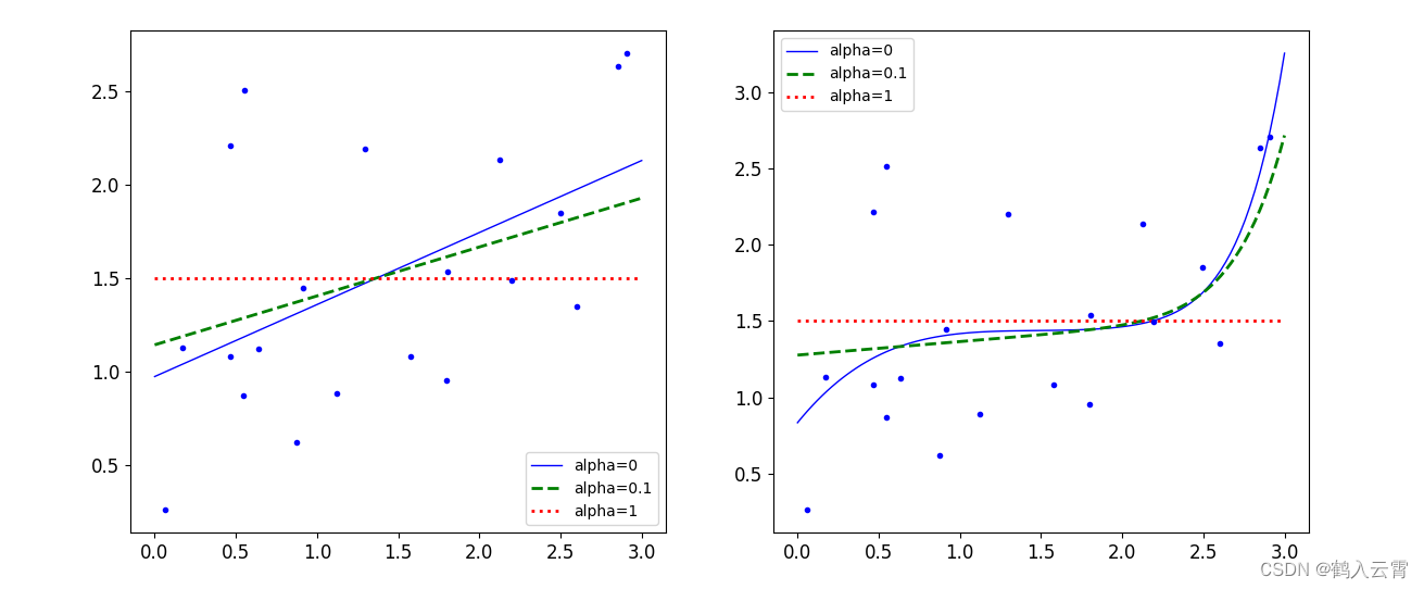
plt.show()

lasso

python 复制代码

from sklearn.linear_model import Lasso
plt.figure(figsize=(14, 6))
plt.subplot(121)
plot_model(Lasso, polynomial=False, alphas=(0, 0.1, 1))
plt.subplot(122)
plot_model(Lasso, polynomial=True, alphas=(0, 10 ** -1, 1))
plt.show()

实验总结

多做实验，得出结果！！！

模型评估方法

sklearn工具包api文档：https://scikit-learn.org/stable/ 现用现查！

交叉验证

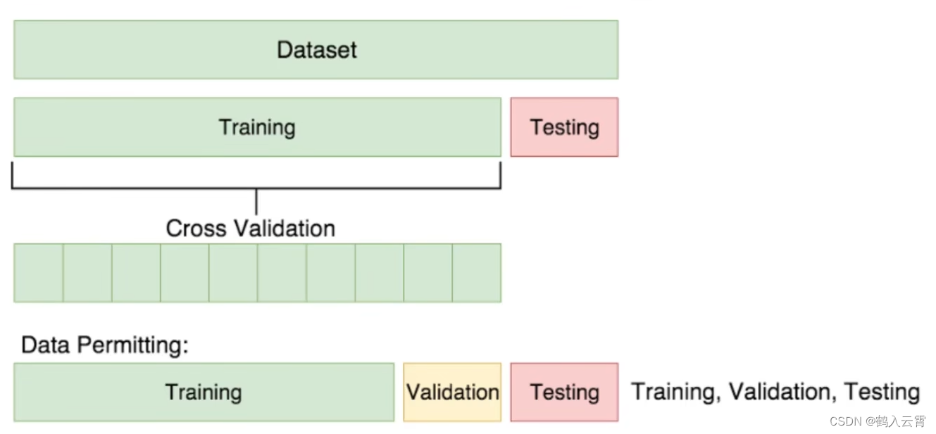
训练集：用于训练模型

验证集：用于评估模型（月考卷）

测试集：用于评估模型（高考卷）

假如训练集被分为5份，验证集就是每次不同的1/5,最终会得到10个模型的准确率，对它们求一个平均值，得到一个比较准确的验证集结果

代码演示

手写数字识别实现

python 复制代码

import numpy as np
import matplotlib.pyplot as plt

# 设置字体大小及相关参数
plt.rcParams['axes.labelsize'] = 14
plt.rcParams['xtick.labelsize'] = 12
plt.rcParams['ytick.labelsize'] = 12
import warnings
warnings.filterwarnings('ignore')  # 忽略sklearn因版本的警告
np.random.seed(42)

# 导入数据
from sklearn.datasets import load_digits
digits = load_digits()
X, y = digits['data'], digits['target']
print(X.shape)
print(y.shape)

# 划分数据集
X_train, X_test, y_train, y_test = X[:1000], X[1000:], y[:1000], y[1000:]

# 洗牌操作 不希望模型学习到数据间由于排序所产生的关系
shuffle_index = np.random.permutation(1000)  # 返回一个长度为1000的数组，其中包含了从0到999的一个随机排列
X_train, y_train = X_train[shuffle_index], y_train[shuffle_index]

y_train_5 = (y_train == 5)
y_test_5 = (y_test == 5)
print(y_train_5[:10])

# 线性回归的梯度下降SGD分类器
from sklearn.linear_model import SGDClassifier
sgd_clf = SGDClassifier(max_iter=5, random_state=42)
sgd_clf.fit(X_train, y_train_5)
print(sgd_clf.predict([X[1000]]))  # 预测值
print(y[1000])  # 真实值

# 交叉验证
from sklearn.model_selection import cross_val_score
# 传入分类器，原始训练集
print(cross_val_score(sgd_clf, X_train, y_train_5, cv=3, scoring='accuracy'))

cross_val_score 自动完成了对训练集验证集的多次切分

手写数字识别实现 (自定义切分训练集验证集+ 克隆)

python 复制代码

import numpy as np
from sklearn.datasets import load_digits
from sklearn.linear_model import SGDClassifier
from sklearn.model_selection import StratifiedKFold  # 对训练集切分
from sklearn.base import clone  # 交叉验证要求每分类器的所有参数都相同


digits = load_digits()
X, y = digits['data'], digits['target']
X_train, X_test, y_train, y_test = X[:1000], X[1000:], y[:1000], y[1000:]
shuffle_index = np.random.permutation(1000)  
X_train, y_train = X_train[shuffle_index], y_train[shuffle_index]

y_train_5 = (y_train == 5)
y_test_5 = (y_test == 5)

sgd_clf = SGDClassifier(max_iter=25, random_state=42)

# 主体：
skflods = StratifiedKFold(n_splits=3, random_state=42, shuffle=True)  # 分3份
for train_index, test_index in skflods.split(X_train, y_train_5):
    # 拿到当前的分类器
    clone_clf = clone(sgd_clf)
    X_train_folds = X_train[train_index]
    y_train_folds = y_train_5[train_index]
    X_test_folds = X_train[test_index]
    y_test_folds = y_train_5[test_index]

    clone_clf.fit(X_train_folds, y_train_folds)
    y_pred = clone_clf.predict(X_test_folds)
    n_correct = sum(y_pred == y_test_folds)
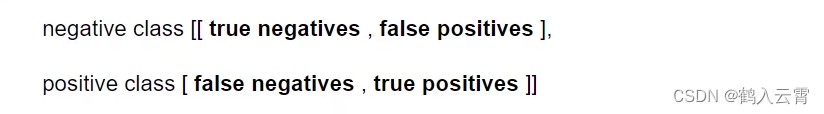
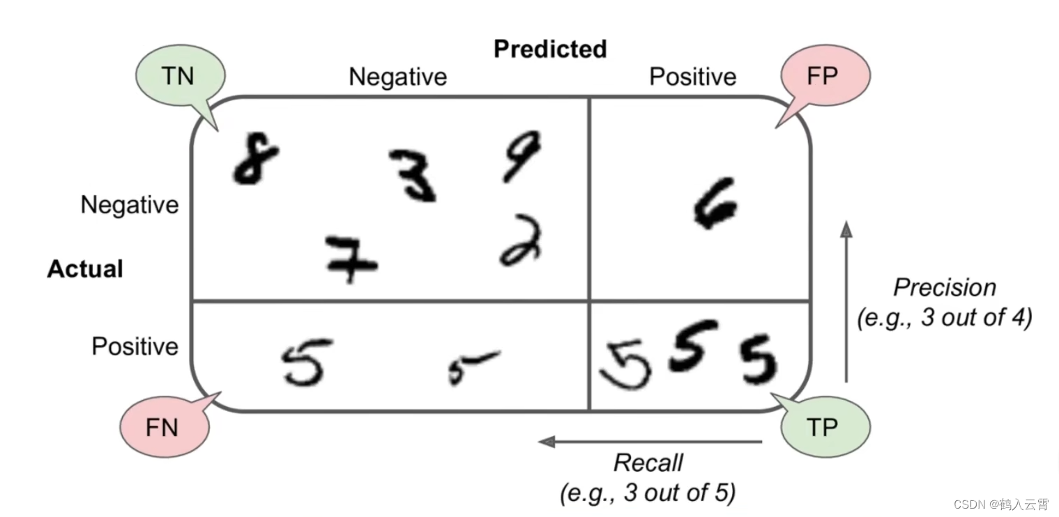
    print(n_correct/len(y_pred))

Confusion Matrix - 混淆矩阵

TP = True Positive = 真阳性

FP = False Positive = 假阳性

FN = False Negative = 假阴性

TN = True Negative = 真阴性

|----|---|----------------|----------------|
| 预测对了预测错了 || 预测 ||
| 预测对了预测错了 || 0 | 1 |
| 真实 | 0 | True Negative | False Positive |
| 真实 | 1 | False Negative | True Positive |

代码演示

python 复制代码

from sklearn.datasets import load_digits
digits = load_digits()
X, y = digits['data'], digits['target']
X_train, X_test, y_train, y_test = X[:1000], X[1000:], y[:1000], y[1000:]
y_train_5 = (y_train == 5)
y_test_5 = (y_test == 5)

from sklearn.linear_model import SGDClassifier
sgd_clf = SGDClassifier(max_iter=30, random_state=42)
sgd_clf.fit(X_train, y_train_5)

from sklearn.model_selection import cross_val_predict
y_train_pred = cross_val_predict(sgd_clf, X_train, y_train_5, cv=3)

# 混淆矩阵
from sklearn.metrics import confusion_matrix
confusion = confusion_matrix(y_train_5, y_train_pred)
print(confusion)

运行结果：

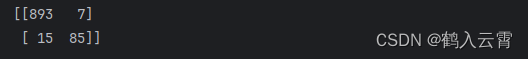
结果解释：

893张被正确的分为非5类别预测：非5 真实：非5

7张被错误的分为5类别预测：5 真实：非5

15张被错误的分为非5类别预测：非5 真实：5

85张被正确的分为5类别预测：5 真实：5

一个完美的分类器应该只有True Positive 和 True Negative ，即主对角线元素不为0,其余元素为0

Precision and Recall - 精度、召回率

查的准不准

查的全不全

sklearn中提供了现成的方法

代码演示

python 复制代码

# 精度、召回率
from sklearn.metrics import precision_score, recall_score
precision = precision_score(y_train_5, y_train_pred)
recall = recall_score(y_train_5, y_train_pred)
print(precision)  # 0.9239130434782609
print(recall)  # 0.85

F1 score (综合评分)

将Precision 和 Recall 结合的一个称为F1 score的指标，调和平均值给予低值更多权重。

因此，如果召回率和精确度都很高，分类器将获得高F1分数

F1 score，反映了模型的稳健型

代码演示

python 复制代码

# F1
from sklearn.metrics import f1_score
f1 = f1_score(y_train_5, y_train_pred)
print(f1)  # 0.8854166666666666

阈值对结果的影响

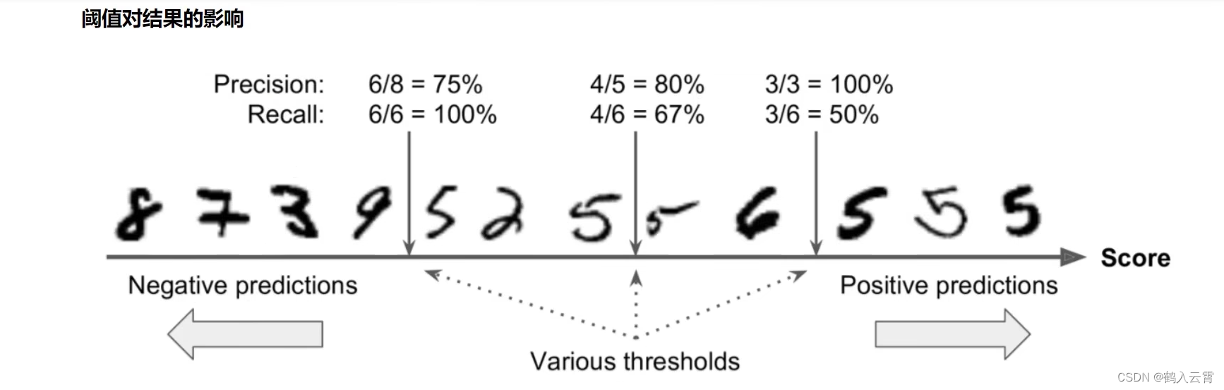
代码解释

python 复制代码

y_score = sgd_clf.decision_function([X[150]])  # 第150个样本
print(y_score)  # [-3016.19616548]
# 自定义阈值
t = 0
y_pred = (y_score > t)
print(y_pred)  # [False]

t = -4000
y_pred = (y_score > t)
print(y_pred)  # [ True]

sklearn中设置阈值

python 复制代码

y_scores = cross_val_predict(sgd_clf, X_train, y_train_5, cv=3, method='decision_function')
# print(y_scores)
from sklearn.metrics import precision_recall_curve
precisions, recalls, thresholds = precision_recall_curve(y_train_5, y_scores)
print(thresholds.shape)  # 会将所有不重复的阈值拿来尝试  # (1000,)
print(precisions.shape)  # (1001,)
print(recalls.shape)    # (1001,)
def plot_precision_recall_vs_threshold(precision, recalls, thresholds):
    plt.plot(thresholds, precision[:-1], 'b--', label='Precision')
    plt.plot(thresholds, recalls[:-1], 'g--', label='Recall')
    plt.xlabel('Threshold', fontsize=16)
    plt.legend(loc='upper left', fontsize=16)
    plt.ylim([0, 1])


plt.figure(figsize=(8, 4))
plot_precision_recall_vs_threshold(precisions, recalls, thresholds)
plt.xlim([-20000, 20000])  # 将x轴的范围设置为从-700000到700000
plt.show()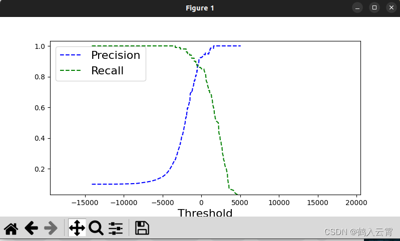

ROC曲线

recelver operating characteristic 是二元分类中的常用评估方法

TPR = TP / (TP + FN)

所有真实类别为1的样本中，预测类别为1的⽐例

FPR = FP / (FP + TN)

所有真实类别为0的样本中，预测类别为1的⽐例

代码演示

python 复制代码

from sklearn.metrics import roc_curve
fpr, tpr, thresholds = roc_curve(y_train_5, y_scores)

def plot_roc_curve(fpr, tpr, label=None):
    plt.plot(fpr, tpr, linewidth=2, label=label)
    plt.plot([0, 1], [0, 1], 'k--')
    plt.axis((0, 1, 0, 1))
    plt.xlabel('False Positive Rate', fontsize=16)
    plt.xlabel('True Positive Rate', fontsize=16)

plt.figure(figsize=(8, 6))
plot_roc_curve(fpr, tpr)
plt.show()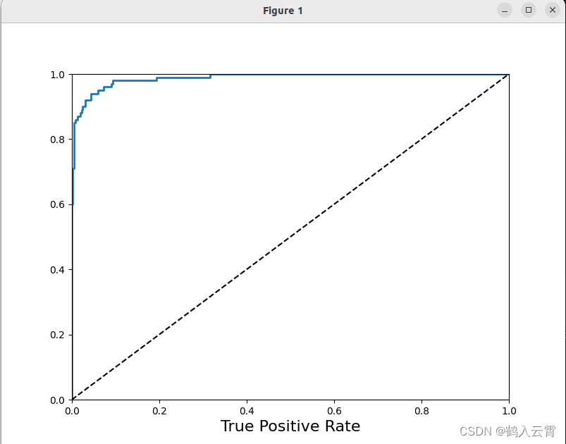

虚线表示纯随机分类器（瞎蒙）的roc曲线；一个好的分类器尽可能远离该线（朝左上角）

比较分类器的一种方法是测量曲线下面积（AUC）。完美分类器的ROC AUC 等于1，而纯随机分类器的ROC AUC 等于0.5, sklearn中提供计算ROC AUC 的函数：

python 复制代码

from sklearn.metrics import roc_auc_score
auc = roc_auc_score(y_train_5, y_scores)
print(auc)  # 0.9886222222222222

逻辑回归

逻辑回归（Logistic Regression）是机器学习中的⼀种分类模型，逻辑回归是⼀种分类算法，虽然名字中带有回归。由于算法的简单和⾼效，在实际中应⽤⾮常⼴泛。

机器学习笔记

引入

问题概述

线性回归

介绍：

误差项定义：

参数求解：

梯度下降：

批量梯度下降：

随机梯度下降：

小批度梯度下降：

线性回归整体模块实现

linear_regression.py 线性回归算法模型

补充

utils.features.normalize.py 标准化

补充

utils.features.prepare_for_training.py 数据预处理

UnivariataLinearRegression.py 线性回归应用（单特征）

补充

MultivariateLinearRegression.py 线性回归应用（多特征）

补充

非线性模型实现

prepare_for_training.py

generate_polynomials.py

generate_sinusoids.py

补充

Non-linearRegression.py

线性回归实验分析

主要内容：

线性回归方程实现

参数直接求解法（非机器学习思想）

使用sklearn工具包实现（机器学习思想：学习的过程即梯度下降）

数据预处理对结果的影响

标准化

梯度下降模块

批量梯度下降 （BGD）

学习率对结果的影响

随机梯度下降（SGD）

小批度梯度下降（MinniBatch）

多项式回归

数据样本数量对结果的影响

正则化

岭回归

lasso

实验总结

模型评估方法

交叉验证

代码演示

手写数字识别实现

手写数字识别实现 (自定义切分训练集验证集+ 克隆)

Confusion Matrix - 混淆矩阵

代码演示

Precision and Recall - 精度、召回率

代码演示

F1 score (综合评分)

代码演示

阈值对结果的影响

代码解释

sklearn中设置阈值

ROC曲线

代码演示

逻辑回归

批量梯度下降（BGD）