大模型强化学习总结

将强化学习应用于强大的基础模型，并结合已经验证的奖励机制，能够显著提升模型的推理能力和性能。Deepseek-R1、Kimi K1.5均是通过策略梯度算法训练而成的。

基本概念

策略 & 动作 & 状态

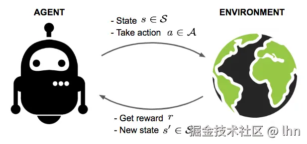
具有参数 <math xmlns="http://www.w3.org/1998/Math/MathML"> θ \theta </math>θ的因果语言模型基于当前文本前缀 <math xmlns="http://www.w3.org/1998/Math/MathML"> s t s_t </math>st(即状态/观测值)，定义下一个token <math xmlns="http://www.w3.org/1998/Math/MathML"> a t ∈ V a_t\in V </math>at∈V的概率分布。在强化学习的情境下，将下一个token <math xmlns="http://www.w3.org/1998/Math/MathML"> a t a_t </math>at 视为一个动作，将当前文本前缀 <math xmlns="http://www.w3.org/1998/Math/MathML"> s t s_t </math>st 视为状态。所以，该语言模型是一个类别型的随机策略。
<math xmlns="http://www.w3.org/1998/Math/MathML" display="block"> a t ∼ π θ ( ⋅ ∣ s t ) , π θ ( a t ∣ s t ) = [ s o f t m a x ( f θ ( s t ) ) ] a t a_t\sim\pi_\theta(\cdot\mid s_t),\quad\pi_\theta(a_t\mid s_t)=\left[\mathrm{softmax}\left(f_\theta(s_t)\right)\right]_{a_t} </math>at∼πθ(⋅∣st),πθ(at∣st)=[softmax(fθ(st))]at

在使用策略梯度优化策略时，需要两种基本操作。

从策略中采样：从上式的类别分布中抽取动作。
为动作的对数似然评分：计算 <math xmlns="http://www.w3.org/1998/Math/MathML"> l o g π θ ( a t ∣ s t ) \mathrm{log}\pi_\theta(a_t\mid s_t) </math>logπθ(at∣st)，用于衡量动作在当前策略下的"合理性"。

在使用LLMs进行强化学习时， <math xmlns="http://www.w3.org/1998/Math/MathML"> s t s_t </math>st指的是到目前为止生成的completion/solution。即模型已输出的文本前缀。每一个 <math xmlns="http://www.w3.org/1998/Math/MathML"> a t a_t </math>at是该solution的下一个token。当文本结束标记（例如<|end_of_text|>）出现时，这个交互过程（episode）就会结束。

轨迹

轨迹（Trajectory）是指智能体所经历的状态和动作的交错序列。
<math xmlns="http://www.w3.org/1998/Math/MathML" display="block"> τ = ( s 0 , a 0 , s 1 , a 1 , ... , s T , a T ) \tau=\left(s_0,a_0,s_1,a_1,\ldots,s_T,a_T\right) </math>τ=(s0,a0,s1,a1,...,sT,aT)

其中， <math xmlns="http://www.w3.org/1998/Math/MathML"> T T </math>T是轨迹的长度。即 <math xmlns="http://www.w3.org/1998/Math/MathML"> a T a_T </math>aT是文本结束标记或者达到最大生成token数量时生成的token。初始状态 <math xmlns="http://www.w3.org/1998/Math/MathML"> s 0 s_0 </math>s0是从初始分布中采样得到的。即 <math xmlns="http://www.w3.org/1998/Math/MathML"> s 0 ∼ ρ 0 ( s 0 ) s_0\sim\rho_0(s_0) </math>s0∼ρ0(s0)；在基于LLMs的强化学习情境下，初始分布 <math xmlns="http://www.w3.org/1998/Math/MathML"> ρ 0 ( s 0 ) \rho_0(s_0) </math>ρ0(s0)是格式化后提示词的分布。

一般情境下，状态转移遵循环境动态 <math xmlns="http://www.w3.org/1998/Math/MathML"> s t + 1 ∼ P ( ⋅ ∣ s t , a t ) s_{t+1}\sim P(\cdot\mid s_t,a_t) </math>st+1∼P(⋅∣st,at)，即下一个状态 <math xmlns="http://www.w3.org/1998/Math/MathML"> s t + 1 s_{t+1} </math>st+1并非完全确定。然而在基于LLMs的RL中，环境是确定性的：下一个状态是由当前状态（即已生成的文本前缀 <math xmlns="http://www.w3.org/1998/Math/MathML"> s t s_t </math>st）和模型生成的token（即动作 <math xmlns="http://www.w3.org/1998/Math/MathML"> a t a_t </math>at）直接拼接而成，
<math xmlns="http://www.w3.org/1998/Math/MathML" display="block"> s t + 1 = s t ∥ a t s_{t+1}=s_t\|a_t </math>st+1=st∥at

轨迹（Trajectories）也可称为episodes（回合）或rollouts（采样序列）。

奖励与回报

奖励是一个标量值 ，用来评判智能体在状态 <math xmlns="http://www.w3.org/1998/Math/MathML"> s t s_t </math>st下执行动作的即时质量。记作 <math xmlns="http://www.w3.org/1998/Math/MathML"> r t = R ( s t , a t ) r_t=R(s_t,a_t) </math>rt=R(st,at)，也称为单步奖励。在需要验证结果的任务（例如数学推理）中，通常将中间步骤的奖励设为0，仅对最终的动作赋予验证奖励。
<math xmlns="http://www.w3.org/1998/Math/MathML" display="block"> r T = R ( s T , a T ) : = { 1 如果生成的完整内容与真实答案匹配 0 otherwise. r_T=R(s_T,a_T):= \begin{cases} 1 & \text{如果生成的完整内容与真实答案匹配} \\ 0 & \text{otherwise.} \end{cases} </math>rT=R(sT,aT):={10如果生成的完整内容与真实答案匹配otherwise.

回报（return）是对一条轨迹上的所有奖励的汇总；有两种计算方式。有限时域（finite-horizon）无折扣回报：适用于有明确终止点的任务。
<math xmlns="http://www.w3.org/1998/Math/MathML" display="block"> R ( τ ) : = ∑ t = 0 r t R(\tau):=\sum_{t=0}r_t </math>R(τ):=t=0∑rt

无限（infinite-horizon）时域折扣回报：通过折扣因子降低远期奖励的权重，适用于无明确终止点的场景。
<math xmlns="http://www.w3.org/1998/Math/MathML" display="block"> R ( τ ) : = ∑ t = 0 ∞ γ t r t , 0 < γ < 1 R(\tau):=\sum_{t=0}^{\infty}\gamma^{t}r_{t},\quad0<\gamma<1 </math>R(τ):=t=0∑∞γtrt,0<γ<1

由于语言模型生成文本有自然终止点（如文本结束标记或最大生成长度），因此采用无折扣的公式。

策略梯度算法

智能体的目标是最大化期望回报。
<math xmlns="http://www.w3.org/1998/Math/MathML" display="block"> J ( θ ) = E τ ∼ π θ [ R ( τ ) ] J(\theta)=\mathbb{E}{\tau\sim\pi\theta}\left[R(\tau)\right] </math>J(θ)=Eτ∼πθ[R(τ)]

上式表示对策略生成的所有可能轨迹的期望（平均值）。对应的优化问题。
<math xmlns="http://www.w3.org/1998/Math/MathML" display="block"> θ ∗ = arg ⁡ max ⁡ θ J ( θ ) \theta^*=\arg\max_\theta J(\theta) </math>θ∗=argθmaxJ(θ)

通过梯度上升优化策略参数 <math xmlns="http://www.w3.org/1998/Math/MathML"> θ \theta </math>θ，以期最大化期望回报。
<math xmlns="http://www.w3.org/1998/Math/MathML" display="block"> θ k + 1 = θ k + α ∇ θ J ( θ k ) \theta_{k+1}=\theta_k+\alpha\nabla_\theta J(\theta_k) </math>θk+1=θk+α∇θJ(θk)

其中, <math xmlns="http://www.w3.org/1998/Math/MathML"> α \alpha </math>α 为学习率, <math xmlns="http://www.w3.org/1998/Math/MathML"> ∇ θ J ( θ k ) \nabla_{\theta} J(\theta_{k}) </math>∇θJ(θk) 是目标函数在当前参数 <math xmlns="http://www.w3.org/1998/Math/MathML"> θ k \theta_{k} </math>θk 处的梯度。核心公式为REINFORCE策略梯度公式，如下：
<math xmlns="http://www.w3.org/1998/Math/MathML" display="block"> ∇ θ J ( π θ ) = E τ ∼ π θ [ ∑ t = 0 T ∇ θ log ⁡ π θ ( a t ∣ s t ) ⋅ R ( τ ) ] \nabla_\theta J(\pi_\theta)=\mathbb{E}{\tau\sim\pi\theta}\left[\sum_{t=0}^T\nabla_\theta\log\pi_\theta(a_t|s_t)\cdot R(\tau)\right] </math>∇θJ(πθ)=Eτ∼πθ[t=0∑T∇θlogπθ(at∣st)⋅R(τ)]

该公式适合于任何可微的 策略，以及任何策略目标函数。

因此，策略梯度等于 "轨迹上所有动作的对数概率梯度" 与 "该轨迹的总回报 <math xmlns="http://www.w3.org/1998/Math/MathML"> R ( τ ) R(\tau) </math>R(τ)" 乘积的期望。若一条轨迹的回报 <math xmlns="http://www.w3.org/1998/Math/MathML"> R ( τ ) R(\tau) </math>R(τ)较高，梯度会增加该轨迹中所有动作的对数概率（使这些动作更易被采样）；若回报较低，则降低对应动作的对数概率。

策略梯度的推导

轨迹的概率（由初始状态分布、环境转移概率和策略共同决定）

<math xmlns="http://www.w3.org/1998/Math/MathML" display="block"> P ( τ ∣ θ ) = ρ 0 ( s 0 ) ∏ t = 0 T P ( s t + 1 ∣ s t , a t ) π θ ( a t ∣ s t ) P(\tau\mid\theta)=\rho_0(s_0)\prod_{t=0}^TP(s_{t+1}\mid s_t,a_t)\pi_\theta(a_t\mid s_t) </math>P(τ∣θ)=ρ0(s0)t=0∏TP(st+1∣st,at)πθ(at∣st)

因此，轨迹的对数概率为
<math xmlns="http://www.w3.org/1998/Math/MathML" display="block"> log ⁡ P ( τ ∣ θ ) = log ⁡ ρ 0 ( s 0 ) + ∑ t = 0 T [ log ⁡ P ( s t + 1 ∣ s t , a t ) + log ⁡ π θ ( a t ∣ s t ) ] \log P(\tau\mid\theta)=\log\rho_0(s_0)+\sum_{t=0}^T\left[\log P(s_{t+1}\mid s_t,a_t)+\log\pi_\theta(a_t\mid s_t)\right] </math>logP(τ∣θ)=logρ0(s0)+t=0∑T[logP(st+1∣st,at)+logπθ(at∣st)]

对数导数技巧 <math xmlns="http://www.w3.org/1998/Math/MathML"> ∇ θ P ( x ; θ ) = P ( x ; θ ) ⋅ ∇ θ log ⁡ P ( x ; θ ) \nabla_\theta P(x;\theta)=P(x;\theta)\cdot\nabla_\theta\log P(x;\theta) </math>∇θP(x;θ)=P(x;θ)⋅∇θlogP(x;θ)
环境相关的量与策略参数无关。 <math xmlns="http://www.w3.org/1998/Math/MathML"> ρ 0 , P ( ⋅ ∣ ⋅ ) \rho_0,P(\cdot\mid\cdot) </math>ρ0,P(⋅∣⋅)与 <math xmlns="http://www.w3.org/1998/Math/MathML"> R ( τ ) R(\tau) </math>R(τ)不依赖策略参数。

<math xmlns="http://www.w3.org/1998/Math/MathML" display="block"> ∇ θ ρ 0 = ∇ θ P = ∇ θ R ( τ ) = 0 \nabla_\theta\rho_0=\nabla_\theta P=\nabla_\theta R(\tau)=0 </math>∇θρ0=∇θP=∇θR(τ)=0

其中， <math xmlns="http://www.w3.org/1998/Math/MathML"> ρ 0 \rho_0 </math>ρ0为初始状态分布（如语言模型任务重"输入文本的分布"）； <math xmlns="http://www.w3.org/1998/Math/MathML"> P ( ⋅ ∣ ⋅ ) P(\cdot\mid\cdot) </math>P(⋅∣⋅)为环境转移概率（如"给定当前状态 <math xmlns="http://www.w3.org/1998/Math/MathML"> s t s_t </math>st和动作 <math xmlns="http://www.w3.org/1998/Math/MathML"> a t a_t </math>at，下一个状态 <math xmlns="http://www.w3.org/1998/Math/MathML"> s t + 1 s_{t+1} </math>st+1出现的概率"）； <math xmlns="http://www.w3.org/1998/Math/MathML"> R ( τ ) R(\tau) </math>R(τ)为轨迹(\tau)的总回报。于是，
<math xmlns="http://www.w3.org/1998/Math/MathML" display="block"> ∇ θ J ( θ ) = ∇ θ E τ ∼ π θ [ R ( τ ) ] = ∇ θ ∑ τ P ( τ ∣ θ ) R ( τ ) = ∑ τ ∇ θ P ( τ ∣ θ ) R ( τ ) = ∑ τ P ( τ ∣ θ ) ∇ θ log ⁡ P ( τ ∣ θ ) R ( τ ) = E τ ∼ π θ [ ∇ θ log ⁡ P ( τ ∣ θ ) R ( τ ) ] \begin{aligned} \nabla_\theta J(\theta) & =\nabla_\theta\mathbb{E}{\tau\sim\pi\theta}[R(\tau)] \\ & =\nabla_\theta\sum_\tau P(\tau|\theta)R(\tau) \\ & =\sum_\tau\nabla_\theta P(\tau|\theta)R(\tau) \\ & =\sum_\tau P(\tau|\theta)\nabla_\theta\log P(\tau|\theta)R(\tau) \\ & =\mathbb{E}{\tau\sim\pi\theta}[\nabla_\theta\log P(\tau|\theta)R(\tau)] \end{aligned} </math>∇θJ(θ)=∇θEτ∼πθ[R(τ)]=∇θτ∑P(τ∣θ)R(τ)=τ∑∇θP(τ∣θ)R(τ)=τ∑P(τ∣θ)∇θlogP(τ∣θ)R(τ)=Eτ∼πθ[∇θlogP(τ∣θ)R(τ)]

期望 <math xmlns="http://www.w3.org/1998/Math/MathML"> E [ ⋅ ] \mathbb{E}[\cdot] </math>E[⋅]在离散情况下可表示为 "所有可能结果的概率 × 结果值" 的总和。这里轨迹 <math xmlns="http://www.w3.org/1998/Math/MathML"> τ \tau </math>τ的概率是 <math xmlns="http://www.w3.org/1998/Math/MathML"> P ( τ ∣ θ ) P(\tau | \theta) </math>P(τ∣θ)（由策略 <math xmlns="http://www.w3.org/1998/Math/MathML"> π θ \pi_{\theta} </math>πθ生成），因此期望展开为所有轨迹的 <math xmlns="http://www.w3.org/1998/Math/MathML"> P ( τ ∣ θ ) ⋅ R ( τ ) P(\tau | \theta) \cdot R(\tau) </math>P(τ∣θ)⋅R(τ)之和。

总梯度等于 "每个轨迹的概率对 θ 的导数" 乘以 "该轨迹回报" 的总和。将梯度重新表示为 "轨迹的函数的期望"，为后续采样估计做准备。

带入轨迹对数概率公式，得到最终的REINFORCE策略梯度公式。

<math xmlns="http://www.w3.org/1998/Math/MathML" display="block"> ∇ θ J ( π θ ) = E τ ∼ π θ [ ∑ t = 0 T ∇ θ log ⁡ π θ ( a t ∣ s t ) R ( τ ) ] \nabla_\theta J(\pi_\theta)=\mathbb{E}{\tau\sim\pi\theta}\left[\sum_{t=0}^T\nabla_\theta\log\pi_\theta(a_t|s_t)R(\tau)\right] </math>∇θJ(πθ)=Eτ∼πθ[t=0∑T∇θlogπθ(at∣st)R(τ)]

对于高回报的轨迹，梯度会 "提升" 该轨迹中所有动作的对数概率；对于低回报的轨迹，则会 "降低" 这些动作的对数概率。

给定一批包含N条轨迹的数据集 <math xmlns="http://www.w3.org/1998/Math/MathML"> D = { τ ( i ) } i = 1 N D = \{\tau^{(i)}\}{i=1}^{N} </math>D={τ(i)}i=1N------ 这些轨迹通过以下方式收集：采样初始状态 <math xmlns="http://www.w3.org/1998/Math/MathML"> s 0 ( i ) ∼ ρ 0 ( s 0 ) s{0}^{(i)} \sim \rho_{0}(s_{0}) </math>s0(i)∼ρ0(s0)，然后在环境中执行策略 <math xmlns="http://www.w3.org/1998/Math/MathML"> π θ \pi_{\theta} </math>πθ，我们可以构造如下无偏梯度估计量：
<math xmlns="http://www.w3.org/1998/Math/MathML" display="block"> g ^ = 1 N ∑ i = 1 N ∑ t = 0 T ∇ θ log ⁡ π θ ( a t ( i ) ∣ s t ( i ) ) R ( τ ( i ) ) \widehat{g}=\frac{1}{N}\sum_{i=1}^N\sum_{t=0}^T\nabla_\theta\log\pi_\theta(a_t^{(i)}\mid s_t^{(i)})R(\tau^{(i)}) </math>g =N1i=1∑Nt=0∑T∇θlogπθ(at(i)∣st(i))R(τ(i))

图形化解释如下：

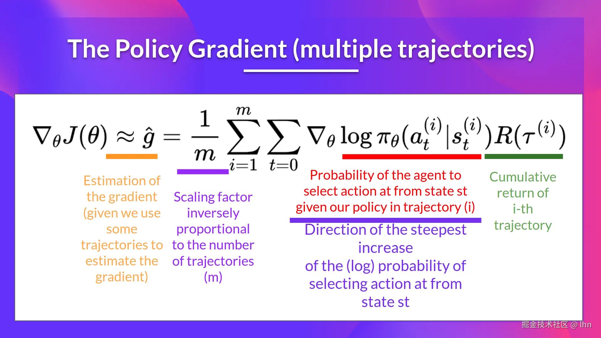
该向量会在梯度上升的参数更新公式 <math xmlns="http://www.w3.org/1998/Math/MathML"> θ ← θ + α g ^ \theta\leftarrow\theta+\alpha\widehat{g} </math>θ←θ+αg 中使用。

Actor-Critic算法

在讲解具体的算法前，先理清一些概念。

状态价值函数

状态价值函数 (state value function) 是指智能体在状态 <math xmlns="http://www.w3.org/1998/Math/MathML"> s t s_t </math>st以及之后的所有时刻都采用策略 <math xmlns="http://www.w3.org/1998/Math/MathML"> π \pi </math>π得到的累计折扣奖励 (回报 )的期望值。是评估状态"好坏"的指标，用于指导智能体决策。
<math xmlns="http://www.w3.org/1998/Math/MathML" display="block"> V π ( s ) = E π [ G t ∣ s t = s ] V_{\boldsymbol{\pi}}(s)=E_{\boldsymbol{\pi}}[G_t|s_t=s] </math>Vπ(s)=Eπ[Gt∣st=s]

其中， <math xmlns="http://www.w3.org/1998/Math/MathML"> V π V_{\boldsymbol{\pi}} </math>Vπ依赖于策略 <math xmlns="http://www.w3.org/1998/Math/MathML"> π \boldsymbol{\pi} </math>π； <math xmlns="http://www.w3.org/1998/Math/MathML"> s t s_t </math>st是指时间 <math xmlns="http://www.w3.org/1998/Math/MathML"> t t </math>t 的当前状态； <math xmlns="http://www.w3.org/1998/Math/MathML"> E π ( ⋅ ) E_\pi(\cdot) </math>Eπ(⋅)上式考虑了所有可能的轨迹（Trajectory）的概率分布，计算期望值； <math xmlns="http://www.w3.org/1998/Math/MathML"> G t G_t </math>Gt是指累计奖励，即从时间步 <math xmlns="http://www.w3.org/1998/Math/MathML"> t t </math>t开始的折扣累计奖励，公式为 <math xmlns="http://www.w3.org/1998/Math/MathML"> G t = r t + γ r t + 1 + γ 2 r t + 2 + ⋯ + γ T − t r T G_t = r_t + \gamma r_{t+1} + \gamma^2 r_{t+2} + \dots + \gamma^{T-t} r_T </math>Gt=rt+γrt+1+γ2rt+2+⋯+γT−trT，且 <math xmlns="http://www.w3.org/1998/Math/MathML"> G t G_t </math>Gt是随机变量，这是由于环境和策略可能具有随机性。

动作价值函数

动作价值函数是指智能体在状态 <math xmlns="http://www.w3.org/1998/Math/MathML"> s t s_t </math>st 采取动作 <math xmlns="http://www.w3.org/1998/Math/MathML"> a t a_t </math>at, 以后的所有时刻都采用策略 <math xmlns="http://www.w3.org/1998/Math/MathML"> π \pi </math>π得到的累计折扣奖励 (回报 )的期望值。它评估了每个状态-动作对 的价值。 <math xmlns="http://www.w3.org/1998/Math/MathML"> Q π ( s , a ) = E π [ G t ∣ s t = s , a t = a ] Q_{\boldsymbol{\pi}}(s,a)=E_{\boldsymbol{\pi}}[G_t|s_t=s,a_t=a] </math>Qπ(s,a)=Eπ[Gt∣st=s,at=a] 其中，动作价值函数也是与策略 <math xmlns="http://www.w3.org/1998/Math/MathML"> π \pi </math>π相关的。

动作价值函数与状态价值函数的关系

\begin{aligned} V_\pi(s_{t}) & =E_{a_{t}\sim\pi(.|s_{t},a_{t})}\[Q_{\pi}(s_{t},a_{t})\] \\ & =\sum_{a_t\in\mathcal{A}}\pi(a_t|s_t)Q_\pi(s_t,a_t) \end{aligned}

<math xmlns="http://www.w3.org/1998/Math/MathML"> V π ( s t ) V_\pi(s_t) </math>Vπ(st) 可以看作智能体在状态 <math xmlns="http://www.w3.org/1998/Math/MathML"> s t s_t </math>st 的"长期价值"，它依赖于智能体可能采取的所有动作 <math xmlns="http://www.w3.org/1998/Math/MathML"> a t a_t </math>at 及其带来的回报。
策略 <math xmlns="http://www.w3.org/1998/Math/MathML"> π \pi </math>π 决定了每个动作的概率， <math xmlns="http://www.w3.org/1998/Math/MathML"> Q π ( s t , a t ) Q_\pi(s_t, a_t) </math>Qπ(st,at) 则提供了执行特定动作后的预期收益。 <math xmlns="http://www.w3.org/1998/Math/MathML"> V π ( s t ) V_\pi(s_t) </math>Vπ(st)本质上是所有可能动作 <math xmlns="http://www.w3.org/1998/Math/MathML"> a a </math>a 的 <math xmlns="http://www.w3.org/1998/Math/MathML"> Q Q </math>Q 值的加权平均，综合反映了所有可能选择的总体效果。也就是 V 是 Q 的期望。

优势函数

优势函数定义了智能体在环境中的某个状态 <math xmlns="http://www.w3.org/1998/Math/MathML"> s s </math>s下采取行动 <math xmlns="http://www.w3.org/1998/Math/MathML"> a a </math>a时，相对于随机采取行动所能获得的额外回报。
<math xmlns="http://www.w3.org/1998/Math/MathML" display="block"> A π ( s , a ) = Q π ( s , a ) − V π ( s ) A^\pi(s,a)=Q^\pi(s,a)-V^\pi(s) </math>Aπ(s,a)=Qπ(s,a)−Vπ(s)

上文提到， <math xmlns="http://www.w3.org/1998/Math/MathML"> V π ( s ) V^\pi(s) </math>Vπ(s) 是"平均预期回报"（根据策略的随机选择），而 <math xmlns="http://www.w3.org/1998/Math/MathML"> Q π ( s , a ) Q^\pi(s,a) </math>Qπ(s,a) 是"特定动作的预期回报"。 <math xmlns="http://www.w3.org/1998/Math/MathML"> V π ( s ) V^\pi(s) </math>Vπ(s) 代表了策略 <math xmlns="http://www.w3.org/1998/Math/MathML"> π \pi </math>π 在状态 <math xmlns="http://www.w3.org/1998/Math/MathML"> s s </math>s 下的"基准线"（baseline），即如果智能体按照策略随机选择动作，能获得的平均收益。减去这个基准，就能突出动作 <math xmlns="http://www.w3.org/1998/Math/MathML"> a a </math>a 的"额外贡献"。

如果 <math xmlns="http://www.w3.org/1998/Math/MathML"> A π ( s , a ) > 0 A^\pi(s,a) > 0 </math>Aπ(s,a)>0：说明执行动作 <math xmlns="http://www.w3.org/1998/Math/MathML"> a a </math>a 的预期回报高于平均水平，这个动作"优于"策略的平均选择。
如果 <math xmlns="http://www.w3.org/1998/Math/MathML"> A π ( s , a ) < 0 A^\pi(s,a) < 0 </math>Aπ(s,a)<0：说明执行动作 <math xmlns="http://www.w3.org/1998/Math/MathML"> a a </math>a 的预期回报低于平均水平，这个动作"劣于"策略的平均选择。
如果 <math xmlns="http://www.w3.org/1998/Math/MathML"> A π ( s , a ) = 0 A^\pi(s,a) = 0 </math>Aπ(s,a)=0：说明执行动作 <math xmlns="http://www.w3.org/1998/Math/MathML"> a a </math>a 的预期回报正好等于平均水平，这个动作"中规中矩"。

注意，这里"随机采取行动"指的是按照策略 <math xmlns="http://www.w3.org/1998/Math/MathML"> π \pi </math>π 的概率分布选择动作，而不是完全均匀随机。

时序差分误差

在单步时序差分方法中，时序差分误差用于更新价值函数。 <math xmlns="http://www.w3.org/1998/Math/MathML"> δ = r t + γ V π θ ( s t + 1 ) − V π θ ( s t ) \delta = r_t+\gamma V^{\pi_\theta}(s_{t+1})-V^{\pi_\theta}(s_t) </math>δ=rt+γVπθ(st+1)−Vπθ(st)

Actor-Critic算法介绍

在上文介绍的REINFORCE策略梯度公式中，目标函数的梯度有一项轨迹回报 <math xmlns="http://www.w3.org/1998/Math/MathML"> R ( τ ) R(\tau) </math>R(τ)，用于指导策略的更新。能否拟和一个价值函数来指导策略进行学习呢？如下图所示。

这正式Actor-Critic算法所做的。我们可以将策略梯度写成更一般的形式：
<math xmlns="http://www.w3.org/1998/Math/MathML" display="block"> ∇ J ( π θ ) = E τ ∼ π θ [ ∑ t = 0 T − 1 Ψ t ∇ l o g π θ ( a t ∣ s t ) ] ≈ 1 N ∑ n = 0 N − 1 ∑ t = 0 T n − 1 Ψ t ∇ l o g π θ ( a t ∣ s t ) \begin{aligned} \nabla J(\pi_{\theta}) & =E_{\tau\sim\pi_{\theta}}[\sum_{t=0}^{T-1}\Psi_{t}\nabla log\pi_{\theta}(a_{t}|s_{t})] \\ & \approx\frac{1}{N}\sum_{n=0}^{N-1}\sum_{t=0}^{T_{n}-1}\Psi_{t}\nabla log\pi_{\theta}(a_{t}|s_{t}) \end{aligned} </math>∇J(πθ)=Eτ∼πθ[t=0∑T−1Ψt∇logπθ(at∣st)]≈N1n=0∑N−1t=0∑Tn−1Ψt∇logπθ(at∣st)

其中， <math xmlns="http://www.w3.org/1998/Math/MathML"> Ψ t \Psi_{t} </math>Ψt的形式有多种：

<math xmlns="http://www.w3.org/1998/Math/MathML"> ∑ t = 0 T r t \sum_{t=0}^Tr_{t} </math>∑t=0Trt：轨迹的总回报。
<math xmlns="http://www.w3.org/1998/Math/MathML"> ∑ t ′ = t T r t ′ \sum_{t^{\prime}=t}^Tr_{t^{\prime}} </math>∑t′=tTrt′：动作 <math xmlns="http://www.w3.org/1998/Math/MathML"> a t a_t </math>at之后的回报。
<math xmlns="http://www.w3.org/1998/Math/MathML"> ∑ t ′ = t T r t ′ − b ( s t ) \sum_{t^{\prime}=t}^Tr_{t^{\prime}}-b(s_t) </math>∑t′=tTrt′−b(st)：基线版本的改进公式。
<math xmlns="http://www.w3.org/1998/Math/MathML"> Q π ( s t , a t ) Q^\pi(s_t,a_t) </math>Qπ(st,at)：动作价值函数。
<math xmlns="http://www.w3.org/1998/Math/MathML"> A π θ ( s t , a t ) A^{\pi_\theta}(s_t,a_t) </math>Aπθ(st,at)：优势函数。
<math xmlns="http://www.w3.org/1998/Math/MathML"> r t + γ V π θ ( s t + 1 ) − V π θ ( s t ) r_t+\gamma V^{\pi_\theta}(s_{t+1})-V^{\pi_\theta}(s_t) </math>rt+γVπθ(st+1)−Vπθ(st)：时序差分误差。

此处讨论的是第六种------时序差分残差 <math xmlns="http://www.w3.org/1998/Math/MathML"> Ψ t = r t + γ V π θ ( s t + 1 ) − V π θ ( s t ) \Psi_{t}=r_t+\gamma V^{\pi_\theta}(s_{t+1})-V^{\pi_\theta}(s_t) </math>Ψt=rt+γVπθ(st+1)−Vπθ(st)来指导策略梯度进行学习。 Actor称为策略网络 ，Critic称为价值网络。

Actor 要做的是与环境交互，并在 Critic 价值函数的指导下用策略梯度学习一个更好的策略。
Critic 要做的是通过 Actor 与环境交互收集的数据学习一个价值函数，这个价值函数会用于判断在当前状态什么动作是好的，什么动作不是好的，进而帮助 Actor 进行策略更新。

Actor的优化目标

Actor ：负责学习并改进策略 <math xmlns="http://www.w3.org/1998/Math/MathML"> π θ ( a ∣ s ) \pi_\theta(a|s) </math>πθ(a∣s)，即在给定状态 <math xmlns="http://www.w3.org/1998/Math/MathML"> s s </math>s 下选择动作 <math xmlns="http://www.w3.org/1998/Math/MathML"> a a </math>a 的概率分布。Actor 的目标是通过调整参数 <math xmlns="http://www.w3.org/1998/Math/MathML"> θ \theta </math>θ，让策略更倾向于选择高回报的动作。

Critic ：负责估计价值函数（如 <math xmlns="http://www.w3.org/1998/Math/MathML"> V π ( s ) V^\pi(s) </math>Vπ(s) 或 <math xmlns="http://www.w3.org/1998/Math/MathML"> Q π ( s , a ) Q^\pi(s, a) </math>Qπ(s,a)），为 Actor 提供反馈，评估当前策略的"好坏"或动作的"优势"（advantage）。

此处，不能忘记Actor的目标仍然是最大化策略的期望回报，即 <math xmlns="http://www.w3.org/1998/Math/MathML"> J ( θ ) = E τ ∼ π θ [ R ( τ ) ] J(\theta)=\mathbb{E}{\tau\sim\pi\theta}\left[R(\tau)\right] </math>J(θ)=Eτ∼πθ[R(τ)]。在 Actor-Critic 中，Actor 的优化目标通常改用优势函数 <math xmlns="http://www.w3.org/1998/Math/MathML"> A π θ ( s t , a t ) A^{\pi_\theta}(s_t,a_t) </math>Aπθ(st,at)替换 <math xmlns="http://www.w3.org/1998/Math/MathML"> R ( τ ) R(\tau) </math>R(τ)来降低方差。公式为
<math xmlns="http://www.w3.org/1998/Math/MathML" display="block"> a r g max ⁡ π θ J ( π θ ) = E τ ∼ π θ [ ∑ t = 0 T A ϕ ( s t , a t ) l o g π θ ( a t ∣ s t ) ] ≈ 1 N ∑ n = 0 N − 1 ∑ t = 0 T n ( r t + γ V ϕ ( s t + 1 ) − V ϕ ( s t ) ) l o g π θ ( a t ∣ s t ) \begin{aligned} arg\max_{\pi_{\theta}}J(\pi_{\theta}) & =E_{\tau\sim\pi_{\theta}}[\sum_{t=0}^{T}A_{\phi}(s_{t},a_{t})log\pi_{\theta}(a_{t}|s_{t})] \\ & \approx\frac{1}{N}\sum_{n=0}^{N-1}\sum_{t=0}^{T_n}(r_t+\gamma V_\phi(s_{t+1})-V_\phi(s_t))log\pi_\theta(a_t|s_t) \end{aligned} </math>argπθmaxJ(πθ)=Eτ∼πθ[t=0∑TAϕ(st,at)logπθ(at∣st)]≈N1n=0∑N−1t=0∑Tn(rt+γVϕ(st+1)−Vϕ(st))logπθ(at∣st)

其中， <math xmlns="http://www.w3.org/1998/Math/MathML"> r t + γ V ϕ ( s t + 1 ) r_t + \gamma V_\phi(s_{t+1}) </math>rt+γVϕ(st+1)：TD 目标（TD target），即即时奖励 <math xmlns="http://www.w3.org/1998/Math/MathML"> r t r_t </math>rt 加上折扣后的下一状态价值 <math xmlns="http://www.w3.org/1998/Math/MathML"> γ V ϕ ( s t + 1 ) \gamma V_\phi(s_{t+1}) </math>γVϕ(st+1)。 <math xmlns="http://www.w3.org/1998/Math/MathML"> γ \gamma </math>γ 是折扣因子（0 ≤ γ < 1），表示对未来奖励的重视程度。

实际上，在单步更新中优势可以由 TD_error 近似（如 <math xmlns="http://www.w3.org/1998/Math/MathML"> A ( s t , a t ) ≈ r t + γ V ( s t + 1 ) − V ( s t ) A(s_t, a_t) \approx r_t + \gamma V(s_{t+1}) - V(s_t) </math>A(st,at)≈rt+γV(st+1)−V(st)）。所以我们不需要等到一个回合（episode）结束后再去优化，而是针对每个时间步 <math xmlns="http://www.w3.org/1998/Math/MathML"> t t </math>t 的状态-动作对 <math xmlns="http://www.w3.org/1998/Math/MathML"> ( s t , a t ) (s_t, a_t) </math>(st,at) 进行调整。也就是说智能体通过在每个时间步上学习，逐步改进策略，而不用等到回合结束。

注：每个时间步 <math xmlns="http://www.w3.org/1998/Math/MathML"> t t </math>t 包括以下过程：

观察状态：智能体接收到环境的当前状态 <math xmlns="http://www.w3.org/1998/Math/MathML"> s t s_t </math>st（比如游戏中的屏幕图像、机器人位置等）。
选择动作：根据策略 <math xmlns="http://www.w3.org/1998/Math/MathML"> π \pi </math>π（或 <math xmlns="http://www.w3.org/1998/Math/MathML"> π θ \pi_\theta </math>πθ），智能体选择一个动作 <math xmlns="http://www.w3.org/1998/Math/MathML"> a t a_t </math>at（比如"向右移动"、"跳跃"）。
执行动作并获得反馈：智能体执行 <math xmlns="http://www.w3.org/1998/Math/MathML"> a t a_t </math>at，环境根据规则返回：
- 即时奖励 <math xmlns="http://www.w3.org/1998/Math/MathML"> r t r_t </math>rt（比如得分 +1 或惩罚 -1）。
- 下一状态 <math xmlns="http://www.w3.org/1998/Math/MathML"> s t + 1 s_{t+1} </math>st+1（环境因动作变化后的新状态）。
重复：进入下一个时间步 <math xmlns="http://www.w3.org/1998/Math/MathML"> t + 1 t+1 </math>t+1，继续这个循环。

Critic的优化目标

Critic承担的角色：（1）价值函数估计：估计智能体在当前策略 <math xmlns="http://www.w3.org/1998/Math/MathML"> π \pi </math>π 下，从某个状态 <math xmlns="http://www.w3.org/1998/Math/MathML"> s s </math>s 开始所能获得的预期累计回报。（2）反馈 Actor：Critic 的估计用于指导 Actor 更新策略。

Critic 的优化目标是使估计的价值函数尽可能接近环境的真实价值函数（true value function）。这通常通过最小化预测值与目标值之间的误差来实现。目标函数通常基于时序差分误差（TD_Error），因为它允许在线学习，而无需等待回合结束。

Critic的优化目标为：
<math xmlns="http://www.w3.org/1998/Math/MathML" display="block"> a r g min ⁡ V ϕ L ( V ϕ ) = E t [ ( r t + γ V ϕ ( s t + 1 ) − V ϕ ( s t ) ) 2 ] arg\min_{V_\phi}L(V_\phi)=E_t[(r_t+\gamma V_\phi(s_{t+1})-V_\phi(s_t))^2] </math>argVϕminL(Vϕ)=Et[(rt+γVϕ(st+1)−Vϕ(st))2]

设当前策略为 <math xmlns="http://www.w3.org/1998/Math/MathML"> π \pi </math>π ，配套价值函数 <math xmlns="http://www.w3.org/1998/Math/MathML"> V π V_\pi </math>Vπ 可精准评估其价值。对于状态 - 动作对 <math xmlns="http://www.w3.org/1998/Math/MathML"> ( s t , a t ) (s_t, a_t) </math>(st,at) ，定义优势函数：
<math xmlns="http://www.w3.org/1998/Math/MathML" display="block"> A π ( s t , a t ) = Q π ( s t , a t ) − V π ( s t ) A_\pi(s_t, a_t) \;=\; Q_\pi(s_t, a_t) \;-\; V_\pi(s_t) </math>Aπ(st,at)=Qπ(st,at)−Vπ(st)

其中， <math xmlns="http://www.w3.org/1998/Math/MathML"> Q π ( s t , a t ) Q_\pi(s_t, a_t) </math>Qπ(st,at) 为"状态 <math xmlns="http://www.w3.org/1998/Math/MathML"> s t s_t </math>st 下执行动作 <math xmlns="http://www.w3.org/1998/Math/MathML"> a t a_t </math>at 的价值期望"（动作价值函数）。若 <math xmlns="http://www.w3.org/1998/Math/MathML"> A π ( s t , a t ) A_\pi(s_t, a_t) </math>Aπ(st,at) 较大，说明 <math xmlns="http://www.w3.org/1998/Math/MathML"> a t a_t </math>at 在 <math xmlns="http://www.w3.org/1998/Math/MathML"> s t s_t </math>st 下"相对更优"，需提升条件概率 <math xmlns="http://www.w3.org/1998/Math/MathML"> π ( a t ∣ s t ) \pi(a_t \vert s_t) </math>π(at∣st) 。通过逐状态调整动作概率分布，最终得到更新策略 <math xmlns="http://www.w3.org/1998/Math/MathML"> π ′ \pi' </math>π′ 。

当且仅当：对任意状态 <math xmlns="http://www.w3.org/1998/Math/MathML"> s t s_t </math>st ，若客观最优动作 <math xmlns="http://www.w3.org/1998/Math/MathML"> a t ∗ a_t^* </math>at∗ 存在，则策略输出 <math xmlns="http://www.w3.org/1998/Math/MathML"> a t ∗ a_t^* </math>at∗ 的条件概率满足：
<math xmlns="http://www.w3.org/1998/Math/MathML" display="block"> π ( a t ∗ ∣ s t ) = 1 （或全局最大概率） \pi(a_t^* \vert s_t) \;=\; 1 \quad \text{（或全局最大概率）} </math>π(at∗∣st)=1（或全局最大概率）

此时策略无提升空间，称 <math xmlns="http://www.w3.org/1998/Math/MathML"> π ′ = π ∗ \pi' = \pi^* </math>π′=π∗ （前提：价值函数 <math xmlns="http://www.w3.org/1998/Math/MathML"> V π V_\pi </math>Vπ 始终精准，可准确度量策略价值）。

当 <math xmlns="http://www.w3.org/1998/Math/MathML"> π ( a t ∗ ∣ s t ) \pi(a_t^* \vert s_t) </math>π(at∗∣st) 取最大值（或 1 ）时，由价值函数与动作价值函数的关系：
<math xmlns="http://www.w3.org/1998/Math/MathML" display="block"> V π ( s t ) = ∑ a ∈ A π ( a ∣ s t ) Q π ( s t , a ) V_\pi(s_t) \;=\; \sum_{a \in \mathcal{A}} \pi(a \vert s_t) \, Q_\pi(s_t, a) </math>Vπ(st)=a∈A∑π(a∣st)Qπ(st,a)

由于 <math xmlns="http://www.w3.org/1998/Math/MathML"> a t ∗ a_t^* </math>at∗ 概率占优， <math xmlns="http://www.w3.org/1998/Math/MathML"> V π ( s t ) V_\pi(s_t) </math>Vπ(st) 会逼近 <math xmlns="http://www.w3.org/1998/Math/MathML"> Q π ( s t , a t ∗ ) Q_\pi(s_t, a_t^*) </math>Qπ(st,at∗) ，因此优势满足：
<math xmlns="http://www.w3.org/1998/Math/MathML" display="block"> A π ( s t , a t ∗ ) = Q π ( s t , a t ∗ ) − V π ( s t ) → 0 A_\pi(s_t, a_t^*) \;=\; Q_\pi(s_t, a_t^*) \;-\; V_\pi(s_t) \;\to\; 0 </math>Aπ(st,at∗)=Qπ(st,at∗)−Vπ(st)→0

解释：优势趋于 0 ，不代表动作"无好坏差异"，而是策略已逼近最优------此时最优动作 <math xmlns="http://www.w3.org/1998/Math/MathML"> a t ∗ a_t^* </math>at∗ 的输出概率天然最大，无需再靠"优势差值"区分。但在策略未收敛阶段 ，优势可有效识别"当前状态下更值得提升的动作"。策略更新为 <math xmlns="http://www.w3.org/1998/Math/MathML"> π ′ \pi' </math>π′ 后，原价值函数 <math xmlns="http://www.w3.org/1998/Math/MathML"> V π V_\pi </math>Vπ 不再适配（因策略分布改变， <math xmlns="http://www.w3.org/1998/Math/MathML"> V π ( s t ) V_\pi(s_t) </math>Vπ(st) 的加权求和基础已变）。需重新拟合价值函数 <math xmlns="http://www.w3.org/1998/Math/MathML"> V π ′ V_{\pi'} </math>Vπ′ ，使其满足：
<math xmlns="http://www.w3.org/1998/Math/MathML" display="block"> V π ′ ( s t ) = ∑ a ∈ A π ′ ( a ∣ s t ) Q π ′ ( s t , a ) V_{\pi'}(s_t) \;=\; \sum_{a \in \mathcal{A}} \pi'(a \vert s_t) \, Q_{\pi'}(s_t, a) </math>Vπ′(st)=a∈A∑π′(a∣st)Qπ′(st,a)

拟合逻辑为：让左侧 <math xmlns="http://www.w3.org/1998/Math/MathML"> V π ′ ( s t ) V_{\pi'}(s_t) </math>Vπ′(st) 匹配右侧新分布的加权结果 ，从而为 <math xmlns="http://www.w3.org/1998/Math/MathML"> π ′ \pi' </math>π′ 构建精准的价值评估体系，支撑下一轮策略迭代。

PPO算法

朴素Actor-Critic算法

<math xmlns="http://www.w3.org/1998/Math/MathML" display="block"> ∇ J ( π θ ) = E t [ A ϕ ( s t , a t ) ∇ l o g π θ ( a t ∣ s t ) ] ≈ 1 N ∗ T ∑ n = 0 N − 1 ∑ t = 0 T n − 1 ( r t + γ V ϕ ( s t + 1 ) − V ϕ ( s t ) ) ∇ l o g π θ ( a t ∣ s t ) \begin{aligned} \nabla J(\pi_{\theta}) & =E_t[A_\phi(s_t,a_t)\nabla log\pi_\theta(a_t|s_t)] \\ & \approx\frac{1}{N*T}\sum_{n=0}^{N-1}\sum_{t=0}^{T_n-1}(r_t+\gamma V_\phi(s_{t+1})-V_\phi(s_t))\nabla log\pi_\theta(a_t|s_t) \end{aligned} </math>∇J(πθ)=Et[Aϕ(st,at)∇logπθ(at∣st)]≈N∗T1n=0∑N−1t=0∑Tn−1(rt+γVϕ(st+1)−Vϕ(st))∇logπθ(at∣st)

注意： <math xmlns="http://www.w3.org/1998/Math/MathML"> ϕ \phi </math>ϕ是Critic网络的参数，但仍需时刻记住 <math xmlns="http://www.w3.org/1998/Math/MathML"> V ϕ V_\phi </math>Vϕ是策略 <math xmlns="http://www.w3.org/1998/Math/MathML"> π \pi </math>π的价值，当策略发生变动时， <math xmlns="http://www.w3.org/1998/Math/MathML"> V ϕ V_\phi </math>Vϕ也会发生变化。

<math xmlns="http://www.w3.org/1998/Math/MathML"> ∇ J ( π θ ) \nabla J(\pi_{\theta}) </math>∇J(πθ)：策略 <math xmlns="http://www.w3.org/1998/Math/MathML"> π θ \pi_\theta </math>πθ 的性能目标 <math xmlns="http://www.w3.org/1998/Math/MathML"> J ( π θ ) J(\pi_\theta) </math>J(πθ)（通常是预期累计回报）对参数 <math xmlns="http://www.w3.org/1998/Math/MathML"> θ \theta </math>θ 的梯度，表示调整 <math xmlns="http://www.w3.org/1998/Math/MathML"> θ \theta </math>θ 能使 <math xmlns="http://www.w3.org/1998/Math/MathML"> J J </math>J 增加的方向。
<math xmlns="http://www.w3.org/1998/Math/MathML"> E t [ ⋅ ] E_t [\cdot] </math>Et[⋅]：对时间步 <math xmlns="http://www.w3.org/1998/Math/MathML"> t t </math>t 的期望，基于策略 <math xmlns="http://www.w3.org/1998/Math/MathML"> π θ \pi_\theta </math>πθ 和环境动态生成的轨迹 <math xmlns="http://www.w3.org/1998/Math/MathML"> ( s t , a t , r t , s t + 1 , ... ) (s_t, a_t, r_t, s_{t+1}, \ldots) </math>(st,at,rt,st+1,...) 计算。
<math xmlns="http://www.w3.org/1998/Math/MathML"> A ϕ ( s t , a t ) A_\phi(s_t, a_t) </math>Aϕ(st,at)：优势函数（advantage function），由 Critic 参数 <math xmlns="http://www.w3.org/1998/Math/MathML"> ϕ \phi </math>ϕ 估计，表示动作 <math xmlns="http://www.w3.org/1998/Math/MathML"> a t a_t </math>at 在状态 <math xmlns="http://www.w3.org/1998/Math/MathML"> s t s_t </math>st 下相对于平均水平的"额外回报"。
<math xmlns="http://www.w3.org/1998/Math/MathML"> ∇ log ⁡ π θ ( a t ∣ s t ) \nabla \log \pi_\theta(a_t | s_t) </math>∇logπθ(at∣st)：策略 <math xmlns="http://www.w3.org/1998/Math/MathML"> π θ \pi_\theta </math>πθ 在状态 <math xmlns="http://www.w3.org/1998/Math/MathML"> s t s_t </math>st 下选择动作 <math xmlns="http://www.w3.org/1998/Math/MathML"> a t a_t </math>at 的对数概率对 <math xmlns="http://www.w3.org/1998/Math/MathML"> θ \theta </math>θ 的梯度，是策略梯度的核心部分。
近似部分：用 <math xmlns="http://www.w3.org/1998/Math/MathML"> N N </math>N 个回合（或批次）中的 <math xmlns="http://www.w3.org/1998/Math/MathML"> T T </math>T 个时间步的样本平均近似期望，具体为：
- <math xmlns="http://www.w3.org/1998/Math/MathML"> 1 N ⋅ T \frac{1}{N \cdot T} </math>N⋅T1：归一化因子， <math xmlns="http://www.w3.org/1998/Math/MathML"> N N </math>N 是回合数， <math xmlns="http://www.w3.org/1998/Math/MathML"> T n T_n </math>Tn 是第 <math xmlns="http://www.w3.org/1998/Math/MathML"> n n </math>n 个回合的时间步数， <math xmlns="http://www.w3.org/1998/Math/MathML"> T T </math>T 是总时间步数的近似平均。
- <math xmlns="http://www.w3.org/1998/Math/MathML"> ∑ n = 0 N − 1 ∑ t = 0 T n − 1 \sum_{n=0}^{N-1} \sum_{t=0}^{T_n-1} </math>∑n=0N−1∑t=0Tn−1：对 <math xmlns="http://www.w3.org/1998/Math/MathML"> N N </math>N 个回合和每个回合的 <math xmlns="http://www.w3.org/1998/Math/MathML"> T n T_n </math>Tn 个时间步求和。
- <math xmlns="http://www.w3.org/1998/Math/MathML"> ( r t + γ V ϕ ( s t + 1 ) − V ϕ ( s t ) ) (r_t + \gamma V_\phi(s_{t+1}) - V_\phi(s_t)) </math>(rt+γVϕ(st+1)−Vϕ(st))：时序差分误差（TD Error），用作优势 <math xmlns="http://www.w3.org/1998/Math/MathML"> A ϕ ( s t , a t ) A_\phi(s_t, a_t) </math>Aϕ(st,at) 的单步估计。
- <math xmlns="http://www.w3.org/1998/Math/MathML"> ∇ log ⁡ π θ ( a t ∣ s t ) \nabla \log \pi_\theta(a_t | s_t) </math>∇logπθ(at∣st)：每个时间步的策略梯度项。

PPO算法实现

在SFT中，我们是去训练模型去模仿给定的一组高质量样本中的响应，然而，这通常不能减轻语言模型在预训练阶段学到的不良行为。对齐语言模型时，从我们试图改进的模型本身获取相应，并根据对这些相应质量和合理性的某种评估给予奖励或惩罚。首先，我们准备一组提示，提供给我们经过SFT之后的模型；然后，从模型中获取针对每个提示的多组相应。（SFT是通过最小化逐个 Token 的交叉熵损失来学习，而是奖励模型去优化一个标量的奖励信号去衡量相应对于给定提示的恰当程度）。 HF是指在原始方法中，这种奖励信号是通过在人类标注的数据上拟合模型得到的，人类会手动对给定的多组相应进行排序。 RLHF 的步骤：

生成相应并获取人类排名：对于每个输入提示，让经过SFT后的模型生成K个不同的响应。然后，人类标注者对这K个相应进行排序。
训练奖励模型（ <math xmlns="http://www.w3.org/1998/Math/MathML"> r θ ( x , y ) r_{\theta}(x,y) </math>rθ(x,y)），对提示-相应对（ <math xmlns="http://www.w3.org/1998/Math/MathML"> x , y x,y </math>x,y）打分，即输出一个标量奖励值。这里奖励模型以SFT模型为基础，移除最后的输出层，并添加一个新的输出层，使其仅输出一个标量值。然后，从人类排名数据集中采样提示以及一对相应 <math xmlns="http://www.w3.org/1998/Math/MathML"> y w , y l y_w,y_l </math>yw,yl，其中 <math xmlns="http://www.w3.org/1998/Math/MathML"> y w y_w </math>yw表示更好的响应， <math xmlns="http://www.w3.org/1998/Math/MathML"> y l y_l </math>yl表示较差的响应（即 <math xmlns="http://www.w3.org/1998/Math/MathML"> y w y_w </math>yw的评分高于 <math xmlns="http://www.w3.org/1998/Math/MathML"> y l y_l </math>yl），优化下面的损失函数。

<math xmlns="http://www.w3.org/1998/Math/MathML" display="block"> ℓ θ r ( x , y w , y l ) = − log ⁡ σ ( r θ ( x , y w ) − r θ ( x , y l ) ) \ell_\theta^r\left(x,y_w,y_l\right)=-\log\sigma\left(r_\theta\left(x,y_w\right)-r_\theta\left(x,y_l\right)\right) </math>ℓθr(x,yw,yl)=−logσ(rθ(x,yw)−rθ(x,yl))

其中， <math xmlns="http://www.w3.org/1998/Math/MathML"> σ \sigma </math>σ是 sigmoid 函数（将差值转换为 0-1 之间的概率）。

我们希望奖励模型输出的标量奖励与人类标注者的排名一致；奖励模型 <math xmlns="http://www.w3.org/1998/Math/MathML"> r r </math>r与人类数据的一致性越高，损失 <math xmlns="http://www.w3.org/1998/Math/MathML"> ℓ r \ell^{r} </math>ℓr就越低。得到奖励模型后，RLHF 通过强化学习（RL）来优化语言模型（LM），此时我们将语言模型视为一个策略 <math xmlns="http://www.w3.org/1998/Math/MathML"> π θ \pi_{\theta} </math>πθ，它接收一个提示并在每一步选择要生成的Token，直到完成响应（结束一个强化学习 "轮次"），此时它会获得由 <math xmlns="http://www.w3.org/1998/Math/MathML"> r θ r_{\theta} </math>rθ给出的奖励。原始论文使用近端策略优化（PPO）算法，借助奖励模型来训练语言模型。此外，在 GPT-3 模型上应用 RLHF 的论文发现，有两点很重要：（a）添加 KL 散度惩罚项，以防止模型与 SFT 基准模型偏离过大；（b）使用预训练（语言建模）目标作为辅助损失函数，以避免下游任务性能退化。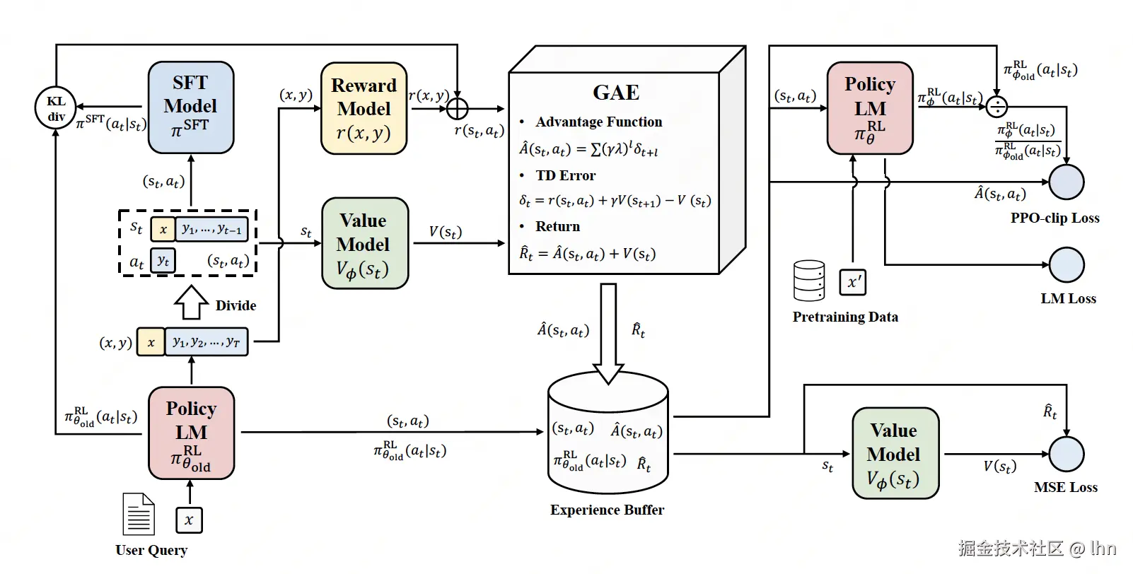图中 Policy LM 是策略（语言）模型，SFT Model 是基准模型，Reward Model 是奖励模型，Value Model 是价值模型。

重要性采样

DPO

在RLHF中，我们首先利用收集到的偏好数据来显式地拟合一个奖励模型 <math xmlns="http://www.w3.org/1998/Math/MathML"> r θ r_{\theta} </math>rθ，然后优化语言模型，使其生成能获得更高奖励的响应。而DPO的出发点是：不必须先找到一个与偏好数据一致的最优奖励模型 <math xmlns="http://www.w3.org/1998/Math/MathML"> r r </math>r，再为该奖励模型找到一个最优策略 <math xmlns="http://www.w3.org/1998/Math/MathML"> π r \pi_r </math>πr。而是，我们可以推导出最优奖励模型的一种重新参数化形式，这种形式可以用最优策略它本身来表示。
<math xmlns="http://www.w3.org/1998/Math/MathML" display="block"> r ( x , y ) = β log ⁡ π r ( y ∣ x ) π r e f ( y ∣ x ) + β log ⁡ Z ( x ) r(x,y)=\beta\log\frac{\pi_r(y|x)}{\pi_\mathrm{ref}(y|x)}+\beta\log Z(x) </math>r(x,y)=βlogπref(y∣x)πr(y∣x)+βlogZ(x)

这里， <math xmlns="http://www.w3.org/1998/Math/MathML"> π ref \pi_{\text{ref}} </math>πref是 "参考策略"：即经过有监督微调（SFT）后的原始语言模型，我们不希望新模型与其偏离过大； <math xmlns="http://www.w3.org/1998/Math/MathML"> β \beta </math>β是一个超参数，用于控制偏离 <math xmlns="http://www.w3.org/1998/Math/MathML"> π ref \pi_{\text{ref}} </math>πref 时的惩罚强度。 <math xmlns="http://www.w3.org/1998/Math/MathML"> π r \pi_{r} </math>πr 是奖励模型 <math xmlns="http://www.w3.org/1998/Math/MathML"> r r </math>r 对应的最优策略 ------ 本质上，就是根据该奖励模型得到的最优语言模型。需要注意的是，式中的第二项仅依赖于一个与指令相关的归一化常数（配分函数 <math xmlns="http://www.w3.org/1998/Math/MathML"> Z ( x ) Z(x) </math>Z(x)），而与补全内容 y 无关。在RLHF中，原始的奖励模型的损失函数仅依赖于两个响应的奖励之差，与单个响应的绝对奖励无关。
<math xmlns="http://www.w3.org/1998/Math/MathML" display="block"> ℓ D P O ( π θ , π r e f , x , y w , y l ) = − log ⁡ σ ( β log ⁡ π θ ( y w ∣ x ) π r e f ( y w ∣ x ) − β log ⁡ π θ ( y l ∣ x ) π r e f ( y l ∣ x ) ) \ell_{\mathrm{DPO}}(\pi_\theta,\pi_{\mathrm{ref}},x,y_w,y_l)=-\log\sigma\left(\beta\log\frac{\pi_\theta(y_w|x)}{\pi_{\mathrm{ref}}(y_w|x)}-\beta\log\frac{\pi_\theta(y_l|x)}{\pi_{\mathrm{ref}}(y_l|x)}\right) </math>ℓDPO(πθ,πref,x,yw,yl)=−logσ(βlogπref(yw∣x)πθ(yw∣x)−βlogπref(yl∣x)πθ(yl∣x))

为计算损失，不需要再对齐过程中对补全内容进行采样，只需要计算条件对数概率即可。所以，这里没有显式的强化学习过程在进行。此外，偏好数据也不一定必须来自人类标注者------可以是来自于其他语言模型生成的偏好数据，这些语言模型通常会被提示根据一系列标准，对同一查询的两组备选响应进行评判。所以，这个过程也不一定涉及人类反馈。

GRPO

群体相对策略优化,英文全称为Group Relative Policy Optimization，简称为GRPO。这是一种策略梯度的变体。

优势估计

群体相对策略优化（GRPO）的核心思想是：从策略 <math xmlns="http://www.w3.org/1998/Math/MathML"> π θ \pi_{\theta} </math>πθ中为每个问题采样多个输出，并利用这些输出计算基线。这种方式十分便捷，因为它避免了学习神经价值函数 <math xmlns="http://www.w3.org/1998/Math/MathML"> V ϕ ( s ) V_{\phi}(s) </math>Vϕ(s)------ 这类函数不仅难以训练，而且从系统角度来看操作繁琐。对于某个问题 <math xmlns="http://www.w3.org/1998/Math/MathML"> q q </math>q以及从 <math xmlns="http://www.w3.org/1998/Math/MathML"> π θ ( ⋅ ∣ q ) \pi_{\theta}(\cdot | q) </math>πθ(⋅∣q)中采样得到的群体输出 <math xmlns="http://www.w3.org/1998/Math/MathML"> { o ( i ) } i = 1 G \{o^{(i)}\}{i=1}^{G} </math>{o(i)}i=1G，令 <math xmlns="http://www.w3.org/1998/Math/MathML"> r ( i ) = R ( q , o ( i ) ) r^{(i)} = R(q, o^{(i)}) </math>r(i)=R(q,o(i))表示第i个输出的奖励。DeepSeekMath（Shao 等人，2024）和 DeepSeek R1（DeepSeek-AI 等人，2025）将第i个输出的群体归一化奖励计算为：
<math xmlns="http://www.w3.org/1998/Math/MathML" display="block"> A ( i ) = r ( i ) − m e a n ( r ( 1 ) , r ( 2 ) , ... , r ( G ) ) s t d ( r ( 1 ) , r ( 2 ) , ... , r ( G ) ) + a d v a n t a g e e p s A^{(i)}=\frac{r^{(i)}-\mathrm{mean}(r^{(1)},r^{(2)},\ldots,r^{(G)})}{\mathrm{std}(r^{(1)},r^{(2)},\ldots,r^{(G)})+\mathrm{advantage}\mathrm{eps}} </math>A(i)=std(r(1),r(2),...,r(G))+advantageepsr(i)−mean(r(1),r(2),...,r(G))

其中， <math xmlns="http://www.w3.org/1998/Math/MathML"> advantage_eps \text{advantage\eps} </math>advantage_eps是一个小常数，用于防止除以零的情况。需要注意的是，该优势值 <math xmlns="http://www.w3.org/1998/Math/MathML"> A ( i ) A^{(i)} </math>A(i)对于响应中的每个 token 都是相同的，即对于所有 <math xmlns="http://www.w3.org/1998/Math/MathML"> t ∈ { 1 , ... , ∣ o ( i ) ∣ } t \in \{1, \ldots, |o^{(i)}|\} </math>t∈{1,...,∣o(i)∣}，都有 <math xmlns="http://www.w3.org/1998/Math/MathML"> A t ( i ) = A ( i ) A{t}^{(i)} = A^{(i)} </math>At(i)=A(i)，因此在后续内容中我们将省略下标 <math xmlns="http://www.w3.org/1998/Math/MathML"> t t </math>t。