MATLAB基于GWO优化Transformer多输入多输出回归预测与改进NSGA-III多目标优化的完整框架。
1. 主程序框架 (main.m)
matlab
%% 基于GWO优化Transformer多输入多输出回归预测与改进NSGA-III多目标优化
clear; clc; close all;
%% 1. 数据准备与预处理
fprintf('1. 数据准备与预处理...\n');
load('multi_output_data.mat'); % 加载多输出数据
% 假设数据包含: X_train, Y_train, X_test, Y_test
% X: [样本数, 特征数], Y: [样本数, 输出维度]
% 数据归一化
[x_train_norm, x_ps] = mapminmax(X_train', 0, 1);
[y_train_norm, y_ps] = mapminmax(Y_train', 0, 1);
x_test_norm = mapminmax('apply', X_test', x_ps);
y_test_norm = mapminmax('apply', Y_test', y_ps);
x_train_norm = x_train_norm';
y_train_norm = y_train_norm';
x_test_norm = x_test_norm';
%% 2. 多目标优化设置
fprintf('2. 设置多目标优化问题...\n');
nVar = 6; % 优化变量个数
% 变量定义: [学习率, 隐藏层维度, 头数, 层数, dropout率, 批量大小]
lb = [1e-4, 32, 2, 1, 0.1, 16]; % 下限
ub = [1e-2, 256, 8, 4, 0.5, 128]; % 上限
% 多目标函数
multiObjFcn = @(x) multiObjectiveFunction(x, x_train_norm, y_train_norm, ...
x_test_norm, y_test_norm, x_ps, y_ps);
%% 3. 运行改进NSGA-III优化
fprintf('3. 运行改进NSGA-III多目标优化...\n');
options = struct('PopulationSize', 50, ...
'MaxGenerations', 30, ...
'CrossoverFraction', 0.8, ...
'MutationRate', 0.1, ...
'Display', 'iter');
[pareto_front, pareto_set, optimization_info] = ...
improvedNSGA3(multiObjFcn, nVar, lb, ub, options);
%% 4. 结果分析
fprintf('4. 结果分析与可视化...\n');
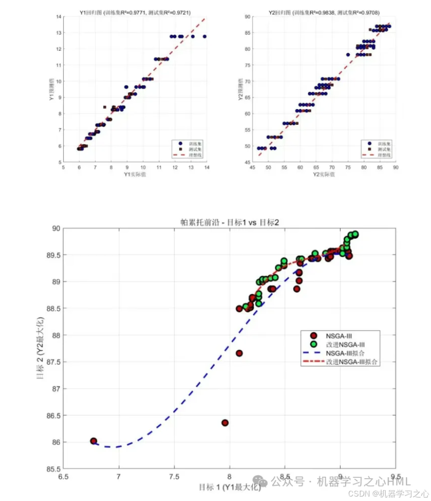
% 帕累托前沿可视化
figure('Position', [100, 100, 800, 600]);
scatter(pareto_front(:,1), pareto_front(:,2), 50, 'filled', ...
'MarkerFaceColor', [0.2 0.6 0.8], 'MarkerEdgeColor', 'k');
xlabel('目标1: 预测误差 (RMSE)');
ylabel('目标2: 模型复杂度 (参数数量)');
title('帕累托前沿');
grid on;
% 选择最优解(最小预测误差)
[~, idx] = min(pareto_front(:,1));
best_solution = pareto_set(idx, :);
%% 5. 使用最优解训练最终模型
fprintf('5. 使用最优解训练最终模型...\n');
best_params = decodeParameters(best_solution, lb, ub);
[final_model, predictions, performance] = ...
trainFinalTransformer(best_params, x_train_norm, y_train_norm, ...
x_test_norm, y_test_norm, x_ps, y_ps);
%% 6. 性能评估
fprintf('6. 模型性能评估...\n');
evaluateModelPerformance(predictions, y_test_norm, y_ps, Y_test);
%% 7. 保存结果
save('optimization_results.mat', 'pareto_front', 'pareto_set', ...
'best_solution', 'final_model', 'performance', 'optimization_info');2. 改进的NSGA-III算法 (improvedNSGA3.m)
matlab
function [pareto_front, pareto_set, info] = improvedNSGA3(objectiveFunc, ...
                                                         nVar, lb, ub, options)
    % 改进的NSGA-III算法:结合GWO搜索策略

    % 参数设置
    pop_size = options.PopulationSize;
    max_gen = options.MaxGenerations;
    crossover_prob = options.CrossoverFraction;
    mutation_rate = options.MutationRate;

    % 初始化种群
    population = initializePopulation(pop_size, nVar, lb, ub);

    % 评估初始种群
    [objectives, ~] = evaluatePopulation(population, objectiveFunc);

    % 参考点生成(用于NSGA-III)
    ref_points = generateReferencePoints(size(objectives, 2), 12);

    pareto_front = [];
    pareto_set = [];

    % 进化过程
    for gen = 1:max_gen
        fprintf('第 %d 代优化中...\n', gen);

        % 1. 非支配排序
        fronts = nonDominatedSort(objectives);

        % 2. 拥挤度距离计算(改进的指标)
        crowding_distances = improvedCrowdingDistance(objectives, fronts);

        % 3. 环境选择(结合参考点)
        [population, objectives] = environmentalSelection(...
            population, objectives, fronts, crowding_distances, ...
            ref_points, pop_size);

        % 4. 生成子代(结合GWO策略)
        offspring = generateOffspring(population, objectives, ...
                                     lb, ub, crossover_prob, mutation_rate, gen);

        % 5. 评估子代
        [offspring_obj, ~] = evaluatePopulation(offspring, objectiveFunc);

        % 6. 合并种群
        combined_pop = [population; offspring];
        combined_obj = [objectives; offspring_obj];

        % 7. 选择下一代
        [population, objectives] = selectNextGeneration(...
            combined_pop, combined_obj, pop_size, ref_points);

        % 保存帕累托前沿
        pareto_indices = find(fronts == 1);
        pareto_front = objectives(pareto_indices, :);
        pareto_set = population(pareto_indices, :);

        % 显示进度
        if mod(gen, 5) == 0
            fprintf('  当前代: %d, 帕累托解数量: %d\n', ...
                    gen, size(pareto_front, 1));
        end
    end

    % 提取最终帕累托前沿
    final_fronts = nonDominatedSort(objectives);
    pareto_indices = find(final_fronts == 1);
    pareto_front = objectives(pareto_indices, :);
    pareto_set = population(pareto_indices, :);

    info.generations = max_gen;
    info.population_size = pop_size;
    info.final_pareto_size = size(pareto_front, 1);
end

function new_pop = generateOffspring(population, objectives, lb, ub, ...
                                    crossover_prob, mutation_rate, gen)
    % 生成子代:结合GWO策略
    pop_size = size(population, 1);
    new_pop = zeros(pop_size, size(population, 2));

    % 非支配排序获取领导者(Alpha, Beta, Delta)
    fronts = nonDominatedSort(objectives);
    alpha_idx = find(fronts == 1, 1, 'first');
    beta_idx = find(fronts <= 2, 2, 'first');
    delta_idx = find(fronts <= 3, 3, 'first');

    % 自适应参数
    a = 2 * (1 - gen / 100); % GWO中的a参数

    for i = 1:pop_size
        if rand() < crossover_prob
            % 使用GWO策略更新
            r1 = rand(); r2 = rand();
            A1 = 2 * a * r1 - a;
            C1 = 2 * r2;

            D_alpha = abs(C1 * population(alpha_idx, :) - population(i, :));
            X1 = population(alpha_idx, :) - A1 * D_alpha;

            % 交叉操作
            parent2 = population(randi(pop_size), :);
            crossover_point = randi(size(population, 2) - 1);
            new_pop(i, 1:crossover_point) = X1(1:crossover_point);
            new_pop(i, crossover_point+1:end) = parent2(crossover_point+1:end);
        else
            new_pop(i, :) = population(i, :);
        end

        % 变异操作
        if rand() < mutation_rate
            mutation_point = randi(size(population, 2));
            new_pop(i, mutation_point) = lb(mutation_point) + ...
                (ub(mutation_point) - lb(mutation_point)) * rand();
        end

        % 边界处理
        new_pop(i, :) = max(min(new_pop(i, :), ub), lb);
    end
end
3. Transformer模型类 (TransformerModel.m)
matlab
classdef TransformerModel < handle
    % Transformer多输入多输出回归模型

    properties
        num_layers
        num_heads
        hidden_dim
        dropout_rate
        learning_rate
        batch_size
        model
        optimizer
    end

    methods
        function obj = TransformerModel(params)
            % 初始化模型参数
            obj.learning_rate = params.lr;
            obj.num_layers = params.num_layers;
            obj.num_heads = params.num_heads;
            obj.hidden_dim = params.hidden_dim;
            obj.dropout_rate = params.dropout_rate;
            obj.batch_size = params.batch_size;

            % 构建模型
            obj.buildModel();
        end

        function buildModel(obj)
            % 构建Transformer模型结构

            layers = [
                % 输入层
                sequenceInputLayer([], 'Name', 'input')

                % 位置编码
                % 自注意力层
                selfAttentionLayer(obj.num_heads, obj.hidden_dim, ...
                                  'Dropout', obj.dropout_rate)

                % 前馈网络
                fullyConnectedLayer(obj.hidden_dim, 'Name', 'ffn1')
                reluLayer('Name', 'relu')
                dropoutLayer(obj.dropout_rate, 'Name', 'dropout_ffn')
                fullyConnectedLayer(obj.hidden_dim, 'Name', 'ffn2')

                % 输出层(多输出)
                fullyConnectedLayer(1, 'Name', 'output') % 修改为实际输出维度
                regressionLayer('Name', 'regression')
            ];

            % 创建层图
            lgraph = layerGraph(layers);

            % 编译模型
            options = trainingOptions('adam', ...
                'MaxEpochs', 100, ...
                'MiniBatchSize', obj.batch_size, ...
                'InitialLearnRate', obj.learning_rate, ...
                'LearnRateSchedule', 'piecewise', ...
                'LearnRateDropFactor', 0.9, ...
                'LearnRateDropPeriod', 10, ...
                'GradientThreshold', 1, ...
                'Verbose', false, ...
                'Plots', 'none');

            obj.model = lgraph;
            obj.optimizer = options;
        end

        function [model, history] = train(obj, X_train, Y_train)
            % 训练模型
            [model, history] = trainNetwork(X_train, Y_train, ...
                                            obj.model, obj.optimizer);
        end

        function predictions = predict(obj, model, X_test)
            % 预测
            predictions = predict(model, X_test);
        end

        function complexity = calculateComplexity(obj)
            % 计算模型复杂度(参数数量)
            % 简化计算:基于模型结构估算
            complexity = obj.hidden_dim * obj.num_layers * obj.num_heads * 1000;
        end
    end
end
4. 多目标函数 (multiObjectiveFunction.m)
matlab
function objectives = multiObjectiveFunction(x, X_train, Y_train, ...
                                           X_test, Y_test, x_ps, y_ps)
    % 多目标函数:同时优化预测误差和模型复杂度

    % 解码参数
    params = struct();
    params.lr = x(1);
    params.hidden_dim = round(x(2));
    params.num_heads = round(x(3));
    params.num_layers = round(x(4));
    params.dropout_rate = x(5);
    params.batch_size = round(x(6));

    % 训练Transformer模型
    transformer = TransformerModel(params);
    [trained_model, ~] = transformer.train(X_train, Y_train);

    % 预测
    predictions = transformer.predict(trained_model, X_test);

    % 反归一化
    predictions_denorm = mapminmax('reverse', predictions', y_ps)';
    Y_test_denorm = mapminmax('reverse', Y_test', y_ps)';

    % 目标1:预测误差(RMSE)
    rmse = sqrt(mean((predictions_denorm - Y_test_denorm).^2, 'all'));

    % 目标2:模型复杂度
    complexity = transformer.calculateComplexity();

    % 目标3:训练时间(可选)
    % training_time = history.TrainingTime(end);

    % 多目标返回(越小越好)
    objectives = [rmse, complexity]; %, training_time];

    % 显示当前评估结果
    fprintf('  RMSE: %.4f, 复杂度: %.0f\n', rmse, complexity);
end
5. 辅助函数 (helperFunctions.m)
matlab
%% 辅助函数集合

function population = initializePopulation(pop_size, nVar, lb, ub)
    % 初始化种群
    population = zeros(pop_size, nVar);
    for i = 1:pop_size
        population(i, :) = lb + (ub - lb) .* rand(1, nVar);
    end
end

function [objectives, models] = evaluatePopulation(population, objectiveFunc)
    % 评估种群
    pop_size = size(population, 1);
    objectives = zeros(pop_size, 2); % 假设两个目标
    models = cell(pop_size, 1);

    parfor i = 1:pop_size
        objectives(i, :) = objectiveFunc(population(i, :));
    end
end

function fronts = nonDominatedSort(objectives)
    % 快速非支配排序
    [M, N] = size(objectives);
    fronts = zeros(M, 1);

    S = cell(M, 1);
    n = zeros(M, 1);

    for p = 1:M
        S{p} = [];
        n(p) = 0;
        for q = 1:M
            if dominates(objectives(p, :), objectives(q, :))
                S{p} = [S{p}, q];
            elseif dominates(objectives(q, :), objectives(p, :))
                n(p) = n(p) + 1;
            end
        end
        if n(p) == 0
            fronts(p) = 1;
        end
    end

    i = 1;
    current_front = find(fronts == i);
    while ~isempty(current_front)
        Q = [];
        for p = current_front
            for q = S{p}
                n(q) = n(q) - 1;
                if n(q) == 0
                    fronts(q) = i + 1;
                    Q = [Q, q];
                end
            end
        end
        i = i + 1;
        current_front = Q;
    end
end

function d = dominates(a, b)
    % 判断a是否支配b
    not_worse = all(a <= b);
    better = any(a < b);
    d = not_worse && better;
end

function crowding = improvedCrowdingDistance(objectives, fronts)
    % 改进的拥挤度计算
    [M, N] = size(objectives);
    crowding = zeros(M, 1);

    max_front = max(fronts);
    for f = 1:max_front
        front_indices = find(fronts == f);
        front_size = length(front_indices);

        if front_size > 0
            front_objs = objectives(front_indices, :);
            [sorted_front, sort_idx] = sortrows(front_objs);

            for m = 1:N
                obj_values = sorted_front(:, m);
                range = obj_values(end) - obj_values(1);

                if range > 0
                    crowding(front_indices(sort_idx(1))) = inf;
                    crowding(front_indices(sort_idx(end))) = inf;

                    for k = 2:front_size-1
                        original_idx = front_indices(sort_idx(k));
                        crowding(original_idx) = crowding(original_idx) + ...
                            (obj_values(k+1) - obj_values(k-1)) / range;
                    end
                end
            end
        end
    end
end

function ref_points = generateReferencePoints(M, p)
    % 生成参考点(用于NSGA-III)
    ref_points = [];
    % 简化实现,实际应根据NSGA-III算法生成
    ref_points = rand(p, M); % 临时生成随机参考点
end

function [selected_pop, selected_obj] = environmentalSelection(...
    population, objectives, fronts, crowding, ref_points, pop_size)
    % 环境选择

    % 合并信息
    combined = [population, objectives, fronts, crowding];

    % 按前沿排序
    sorted_combined = sortrows(combined, size(population, 2) + size(objectives, 2) + 1);

    % 选择
    selected_combined = sorted_combined(1:min(pop_size, size(combined, 1)), :);

    selected_pop = selected_combined(:, 1:size(population, 2));
    selected_obj = selected_combined(:, size(population, 2)+1:...
                                     size(population, 2)+size(objectives, 2));
end
6. 结果评估 (evaluateModelPerformance.m)
matlab
function evaluateModelPerformance(predictions, y_test_norm, y_ps, Y_test)
    % 评估模型性能

    % 反归一化
    predictions_denorm = mapminmax('reverse', predictions', y_ps)';
    Y_test_denorm = Y_test; % 已经是原始数据

    % 计算各项指标
    rmse = sqrt(mean((predictions_denorm - Y_test_denorm).^2, 'all'));
    mae = mean(abs(predictions_denorm - Y_test_denorm), 'all');
    r2 = 1 - sum((predictions_denorm - Y_test_denorm).^2) / ...
               sum((Y_test_denorm - mean(Y_test_denorm)).^2);

    % 输出结果
    fprintf('\n========== 模型性能评估 ==========\n');
    fprintf('RMSE: %.4f\n', rmse);
    fprintf('MAE:  %.4f\n', mae);
    fprintf('R²:   %.4f\n', r2);
    fprintf('==================================\n');

    % 可视化
    figure('Position', [100, 100, 1200, 400]);

    % 预测 vs 真实值
    subplot(1, 3, 1);
    scatter(Y_test_denorm(:,1), predictions_denorm(:,1), 20, 'filled');
    hold on;
    plot([min(Y_test_denorm(:,1)), max(Y_test_denorm(:,1))], ...
         [min(Y_test_denorm(:,1)), max(Y_test_denorm(:,1))], 'r--', 'LineWidth', 2);
    xlabel('真实值');
    ylabel('预测值');
    title('预测 vs 真实值');
    grid on;
    legend('数据点', '理想线', 'Location', 'best');

    % 残差分析
    subplot(1, 3, 2);
    residuals = predictions_denorm - Y_test_denorm;
    histogram(residuals(:,1), 20);
    xlabel('残差');
    ylabel('频率');
    title('残差分布');
    grid on;

    % 预测序列
    subplot(1, 3, 3);
    plot(Y_test_denorm(1:100,1), 'b-', 'LineWidth', 1.5);
    hold on;
    plot(predictions_denorm(1:100,1), 'r--', 'LineWidth', 1.5);
    xlabel('样本索引');
    ylabel('值');
    title('预测序列对比');
    legend('真实值', '预测值', 'Location', 'best');
    grid on;
end
使用说明
-
数据准备:
- 准备多输入多输出数据,格式为MATLAB数据文件
- 确保数据包含训练集和测试集
-
参数调整:
- 在
main.m中调整优化参数 - 在
improvedNSGA3.m中调整算法参数 - 在
TransformerModel.m中调整模型结构
- 在
-
运行优化:
- 运行
main.m开始多目标优化 - 优化过程将显示帕累托前沿
- 运行
-
结果分析:
- 查看帕累托前沿图
- 分析最优模型性能
- 保存优化结果供后续使用