Biseq计算差异甲基化区域

一、写在前面

此前给大家分享了一文掌握WGBS分析流程,为大家进行了背景知识介绍、环境布置、质控、单样本/多样本定量、去重、甲基化提取、DMR、DMS计算注释等操作。这里，我们再演示一种计算差异甲基化区域的工具包：

BiSeq被设计用于重亚硫酸盐测序(bisulfite suquencing)数据的分析，例如reduce representation bisulfite sequencing (RRBS), whole genome bistulfite sequencing (WGBS)。本文分析集锦：

BiSeq最近一次维护在2022.04，大家可以放心大胆的使用：

复制代码

packageDescription('BiSeq')

## Package: BiSeq
## Type: Package
## Title: Processing and analyzing bisulfite sequencing data
## Version: 1.36.0
## Date: 2022-01-14
## Author: Katja Hebestreit, Hans-Ulrich Klein
## Maintainer: Katja Hebestreit <katja.hebestreit@gmail.com>
## Depends: R (>= 3.5.0), methods, S4Vectors, IRanges (>= 1.17.24),
##         GenomicRanges, SummarizedExperiment (>= 0.2.0), Formula
## Imports: methods, BiocGenerics, Biobase, S4Vectors, IRanges,
##         GenomeInfoDb, GenomicRanges, SummarizedExperiment, rtracklayer,
##         parallel, betareg, lokern, Formula, globaltest
## Description: The BiSeq package provides useful classes and functions to
##         handle and analyze targeted bisulfite sequencing (BS) data such
##         as reduced-representation bisulfite sequencing (RRBS) data. In
##         particular, it implements an algorithm to detect differentially
##         methylated regions (DMRs). The package takes already aligned BS
##         data from one or multiple samples.
## License: LGPL-3
## biocViews: Genetics, Sequencing, MethylSeq, DNAMethylation
## git_url: https://git.bioconductor.org/packages/BiSeq
## git_branch: RELEASE_3_15
## git_last_commit: b5cd494
## git_last_commit_date: 2022-04-26
## Date/Publication: 2022-04-26
## NeedsCompilation: no
## Packaged: 2022-04-26 21:40:40 UTC; biocbuild
## Built: R 4.2.0; ; 2022-04-27 09:13:26 UTC; windows
## 
## -- File: D:/R-4.2.1/library/BiSeq/Meta/package.rds

本文测试数据下载：

网盘下载链接: https://pan.baidu.com/s/1ddPPAv2zzy_SGhJezzsvKA

联系客服[Biomamba_yunying]

获取提取码: yp67

二、数据输入

2.1 `BSraw`

2.1.1 快速创建输入数据：

BSraw需要两个输入数据，第一个为Bismark的methylation_extractor生成的.cov文件，第二个colData记录的是分组信息

复制代码

suppressMessages(if(!require(BiSeq))BiocManager::install('BiSeq'))

## Warning: 程辑包'GenomeInfoDb'是用R版本4.2.2 来建造的

## Warning: 'aperm'存在多个方法表

## Warning: replacing previous import 'BiocGenerics::aperm' by
## 'DelayedArray::aperm' when loading 'SummarizedExperiment'

## Warning in .recacheSubclasses(def@className, def, env):
## "vector_OR_Vector"类别的子类别"DataFrameFactor"没有定义；因此没有更新

test.file <-system.file("extdata", "CpG_context_test_sample.cov", package ="BiSeq")
test.file

## [1] "D:/R-4.2.1/library/BiSeq/extdata/CpG_context_test_sample.cov"

#先自行读入
coveragefile <-read.table(test.file)
head(coveragefile)

##      V1    V2    V3        V4 V5 V6
## 1 chr12 60217 60217  71.42857 10  4
## 2 chr12 60218 60218  87.50000  7  1
## 3 chr12 60306 60306  94.11765 16  1
## 4 chr12 60307 60307  80.00000  4  1
## 5 chr12 60381 60381  84.61538 11  2
## 6 chr12 60382 60382 100.00000 16  0

这是一个bismark生成的coverage文件，包含的六列含义分别是：

复制代码

<chromosome><start position><end position><methylation percentage><count methylated><count unmethylated>

rrbs.raw <-readBismark(test.file,
colData=DataFrame(row.names="sample_1"))

## Processing sample sample_1 ... 
## Building BSraw object.

class(rrbs.raw)

## [1] "BSraw"
## attr(,"package")
## [1] "BiSeq"

构建好的是一个BSraw对象，它实际上是一个S4对象，主要包含四个slots:
1、一个包含metadata的list: rrbs.raw@metadata
2、一个包含个样本CpG位点位置信息的GRanges: rrbs.raw@rowRanges
3、一个包含样本信息的DataFrame: rrbs.raw@colData
4、一个包含总reads(totolReads)和甲基化reads(methReads)的assays：rrbs.raw@assays$totalReads和rrbs.raw@assays$methReads

2.1.2 手动创建输入数据

这能帮助大家更好的了解数据格式：

复制代码

#构建metadata:
metadata <-list(Sequencer ="Instrument", Year ="2013")
#构建rowRanges:
rowRanges <-GRanges(seqnames ="chr1",
ranges =IRanges(start =c(1,2,3), end =c(1,2,3)))
#构建colData，大家自行准备一个table读入也可以
colData <-DataFrame(group =c("cancer", "control"),
row.names =c("sample_1", "sample_2"))
#totalReads和methReads实际上是矩阵：
totalReads <-matrix(c(rep(10L, 3), rep(5L, 3)), ncol =2)
methReads <-matrix(c(rep(5L, 3), rep(5L, 3)), ncol =2)

#最后可以合并传递给BSraw函数：  
BSraw(metadata = metadata,
rowRanges = rowRanges,
colData = colData,
totalReads = totalReads,
methReads = methReads)

## class: BSraw 
## dim: 3 2 
## metadata(0):
## assays(2): totalReads methReads
## rownames: NULL
## rowData names(0):
## colnames(2): sample_1 sample_2
## colData names(1): group

2.1.3 测试数据：

BiSeq的输入数据是对比对后结果进行甲基化信息提取的文件，这里的测试数据由Bismark(version 0.5)生成。测试数据是一个十样本(共两组：5个acute promyelocytic leukemia (APL)，5个APL in remission)的rrbs.raw数据，包含染色体1、2的CpG位点信息。

复制代码

data(rrbs)#载入数据
rrbs.raw <- rrbs
#查看数据对象包含内容
colData(rrbs.raw)#等同于rrbs.raw@colData

## DataFrame with 10 rows and 1 column
##             group
##          <factor>
## APL1      APL    
## APL2      APL    
## APL3      APL    
## APL7      APL    
## APL8      APL    
## APL10961  control
## APL11436  control
## APL11523  control
## APL11624  control
## APL5894   control

head(rowRanges(rrbs.raw))#等同于rrbs.raw@rowRanges

## GRanges object with 6 ranges and 0 metadata columns:
##        seqnames    ranges strand
##           <Rle> <IRanges>  <Rle>
##   1456     chr1    870425      +
##   1457     chr1    870443      +
##   1458     chr1    870459      +
##   1459     chr1    870573      +
##   1460     chr1    870584      +
##   1461     chr1    870599      +
##   -------
##   seqinfo: 25 sequences from an unspecified genome; no seqlengths

head(totalReads(rrbs.raw))#等同于rrbs.raw@assays$totalReads

##      APL1 APL2 APL3 APL7 APL8 APL10961 APL11436 APL11523 APL11624 APL5894
## 1456   39    6   10    0    0       48       31       65       39      29
## 1457   39    6   10    0    0       48       31       65       39      29
## 1458   39    6   10    0    0       48       27       65       39      29
## 1459   20   26   49   48   39       27       23       34       29      15
## 1460   20   26   49   48   39       27       23       34       28      15
## 1461   20   26   49   48   39       27       22       34       29      15

head(methReads(rrbs.raw))#等同于rrbs.raw@assays$methReads

##      APL1 APL2 APL3 APL7 APL8 APL10961 APL11436 APL11523 APL11624 APL5894
## 1456   32    6    7    0    0       15       23       16        7       7
## 1457   33    6    7    0    0       18       10       19        2       7
## 1458   33    6   10    0    0       20       10       19        2       3
## 1459   13   20   34   41   32        3        8        8        6       4
## 1460   14   18   35   37   33        2        4        4        3       0
## 1461   14   16   35   40   31        5        5        5        1       2

2.2 `BSrel`

BSrel对象收录的是数据的相对甲基化信息。大部分结构与内容与BSraw类似，不过assays包含的是相对甲基化水平(0至1)，而不是原来的reads数，相当于存放的是methReads/totalReads。

2.2.1 手动创建：

与上面的BSraw几乎没差别

复制代码

methLevel <-matrix(c(rep(0.5, 3), rep(1, 3)), ncol =2)
rrbs.rel <-BSrel(metadata = metadata,
rowRanges = rowRanges,
colData = colData,
methLevel = methLevel)

甚至二者之间可以直接转换：

复制代码

rrbs.rel <-rawToRel(rrbs.raw)
rrbs.rel

## class: BSrel 
## dim: 10502 10 
## metadata(0):
## assays(1): methLevel
## rownames(10502): 1456 1457 ... 4970981 4970982
## rowData names(0):
## colnames(10): APL1 APL2 ... APL11624 APL5894
## colData names(1): group

看一下二者不同的地方：

复制代码

head(rrbs.raw@assays@data$methReads)

##      APL1 APL2 APL3 APL7 APL8 APL10961 APL11436 APL11523 APL11624 APL5894
## 1456   32    6    7    0    0       15       23       16        7       7
## 1457   33    6    7    0    0       18       10       19        2       7
## 1458   33    6   10    0    0       20       10       19        2       3
## 1459   13   20   34   41   32        3        8        8        6       4
## 1460   14   18   35   37   33        2        4        4        3       0
## 1461   14   16   35   40   31        5        5        5        1       2

head(rrbs.raw@assays@data$totalReads)

##      APL1 APL2 APL3 APL7 APL8 APL10961 APL11436 APL11523 APL11624 APL5894
## 1456   39    6   10    0    0       48       31       65       39      29
## 1457   39    6   10    0    0       48       31       65       39      29
## 1458   39    6   10    0    0       48       27       65       39      29
## 1459   20   26   49   48   39       27       23       34       29      15
## 1460   20   26   49   48   39       27       23       34       28      15
## 1461   20   26   49   48   39       27       22       34       29      15

head(rrbs.rel@assays@data$methLevel)

##           APL1      APL2      APL3      APL7      APL8   APL10961  APL11436
## 1456 0.8205128 1.0000000 0.7000000       NaN       NaN 0.31250000 0.7419355
## 1457 0.8461538 1.0000000 0.7000000       NaN       NaN 0.37500000 0.3225806
## 1458 0.8461538 1.0000000 1.0000000       NaN       NaN 0.41666667 0.3703704
## 1459 0.6500000 0.7692308 0.6938776 0.8541667 0.8205128 0.11111111 0.3478261
## 1460 0.7000000 0.6923077 0.7142857 0.7708333 0.8461538 0.07407407 0.1739130
## 1461 0.7000000 0.6153846 0.7142857 0.8333333 0.7948718 0.18518519 0.2272727
##       APL11523   APL11624   APL5894
## 1456 0.2461538 0.17948718 0.2413793
## 1457 0.2923077 0.05128205 0.2413793
## 1458 0.2923077 0.05128205 0.1034483
## 1459 0.2352941 0.20689655 0.2666667
## 1460 0.1176471 0.10714286 0.0000000
## 1461 0.1470588 0.03448276 0.1333333

#所以理论上应有以下等式
head(rrbs.raw@assays@data$methReads)/head(rrbs.raw@assays@data$totalReads)==head(rrbs.rel@assays@data$methLevel)

##      APL1 APL2 APL3 APL7 APL8 APL10961 APL11436 APL11523 APL11624 APL5894
## 1456 TRUE TRUE TRUE   NA   NA     TRUE     TRUE     TRUE     TRUE    TRUE
## 1457 TRUE TRUE TRUE   NA   NA     TRUE     TRUE     TRUE     TRUE    TRUE
## 1458 TRUE TRUE TRUE   NA   NA     TRUE     TRUE     TRUE     TRUE    TRUE
## 1459 TRUE TRUE TRUE TRUE TRUE     TRUE     TRUE     TRUE     TRUE    TRUE
## 1460 TRUE TRUE TRUE TRUE TRUE     TRUE     TRUE     TRUE     TRUE    TRUE
## 1461 TRUE TRUE TRUE TRUE TRUE     TRUE     TRUE     TRUE     TRUE    TRUE

2.3 `BiSeq`对象简单处理

对于BSraw和BSrel来说处理的方式基本相同：

复制代码

dim(rrbs)#返回值为基因数、样本数

## [1] 10502    10

取子集

复制代码

#取出指定基因：
rrbs.raw[,"APL2"]

## class: BSraw 
## dim: 10502 1 
## metadata(0):
## assays(2): totalReads methReads
## rownames(10502): 1456 1457 ... 4970981 4970982
## rowData names(0):
## colnames(1): APL2
## colData names(1): group

#得到对应染色体的坐标：
ind.chr1 <-which(seqnames(rrbs) =="chr1")
ind.chr1[1:5]

## [1] 1 2 3 4 5

#取出指定染色体的数据：
rrbs[ind.chr1,]

## class: BSraw 
## dim: 681 10 
## metadata(0):
## assays(2): totalReads methReads
## rownames(681): 1456 1457 ... 402262 402263
## rowData names(0):
## colnames(10): APL1 APL2 ... APL11624 APL5894
## colData names(1): group

#用基因组的位置取子集也是支持的：
region <-GRanges(seqnames="chr1",
ranges=IRanges(start =875200,
end =875500))

找交集：

复制代码

findOverlaps(rrbs, region)

## Hits object with 21 hits and 0 metadata columns:
##        queryHits subjectHits
##        <integer>   <integer>
##    [1]        77           1
##    [2]        78           1
##    [3]        79           1
##    [4]        80           1
##    [5]        81           1
##    ...       ...         ...
##   [17]       405           1
##   [18]       406           1
##   [19]       407           1
##   [20]       408           1
##   [21]       409           1
##   -------
##   queryLength: 10502 / subjectLength: 1

取交集：

复制代码

subsetByOverlaps(rrbs, region)

## class: BSraw 
## dim: 21 10 
## metadata(0):
## assays(2): totalReads methReads
## rownames(21): 1542 1543 ... 401947 401948
## rowData names(0):
## colnames(10): APL1 APL2 ... APL11624 APL5894
## colData names(1): group

按照CpG在染色体中的位置升序排列：

复制代码

sort(rrbs)

## class: BSraw 
## dim: 10502 10 
## metadata(0):
## assays(2): totalReads methReads
## rownames(10502): 1456 1457 ... 4970981 4970982
## rowData names(0):
## colnames(10): APL1 APL2 ... APL11624 APL5894
## colData names(1): group

BSraw和BSrel对象可以进行合并与拆分：

复制代码

combine(rrbs[1:10,1:2], rrbs[1:1000, 3:10])

## class: BSraw 
## dim: 1000 10 
## metadata(0):
## assays(2): totalReads methReads
## rownames(1000): 1456 1457 ... 4636787 4636788
## rowData names(0):
## colnames(10): APL1 APL2 ... APL11624 APL5894
## colData names(1): group

split(rowRanges(rrbs),
f =as.factor(as.character(seqnames(rrbs))))

## GRangesList object of length 2:
## $chr1
## GRanges object with 681 ranges and 0 metadata columns:
##          seqnames    ranges strand
##             <Rle> <IRanges>  <Rle>
##     1456     chr1    870425      +
##     1457     chr1    870443      +
##     1458     chr1    870459      +
##     1459     chr1    870573      +
##     1460     chr1    870584      +
##      ...      ...       ...    ...
##   402259     chr1    888967      -
##   402260     chr1    889714      -
##   402261     chr1    889729      -
##   402262     chr1    889854      -
##   402263     chr1    889875      -
##   -------
##   seqinfo: 25 sequences from an unspecified genome; no seqlengths
## 
## $chr2
## GRanges object with 9821 ranges and 0 metadata columns:
##           seqnames    ranges strand
##              <Rle> <IRanges>  <Rle>
##   4636394     chr2     43091      +
##   4636395     chr2     43151      +
##   4636397     chr2     45448      +
##   4636400     chr2     45617      +
##   4636401     chr2     45626      +
##       ...      ...       ...    ...
##   4970976     chr2   1999037      -
##   4970979     chr2   1999436      -
##   4970980     chr2   1999446      -
##   4970981     chr2   1999468      -
##   4970982     chr2   1999939      -
##   -------
##   seqinfo: 25 sequences from an unspecified genome; no seqlengths

三、数据分析

3.1 质控

统计个样本CpG位点的覆盖度：

复制代码

covStatistics(rrbs)#统计

## $Covered_CpG_sites
##     APL1     APL2     APL3     APL7     APL8 APL10961 APL11436 APL11523 
##     5217     4240     4276     3972     3821     5089     5169     6922 
## APL11624  APL5894 
##     6483     7199 
## 
## $Median_coverage
##     APL1     APL2     APL3     APL7     APL8 APL10961 APL11436 APL11523 
##       12        5       12       15       11       10        6        8 
## APL11624  APL5894 
##        4        5

covBoxplots(rrbs, col ="cornflowerblue", las =2)#绘图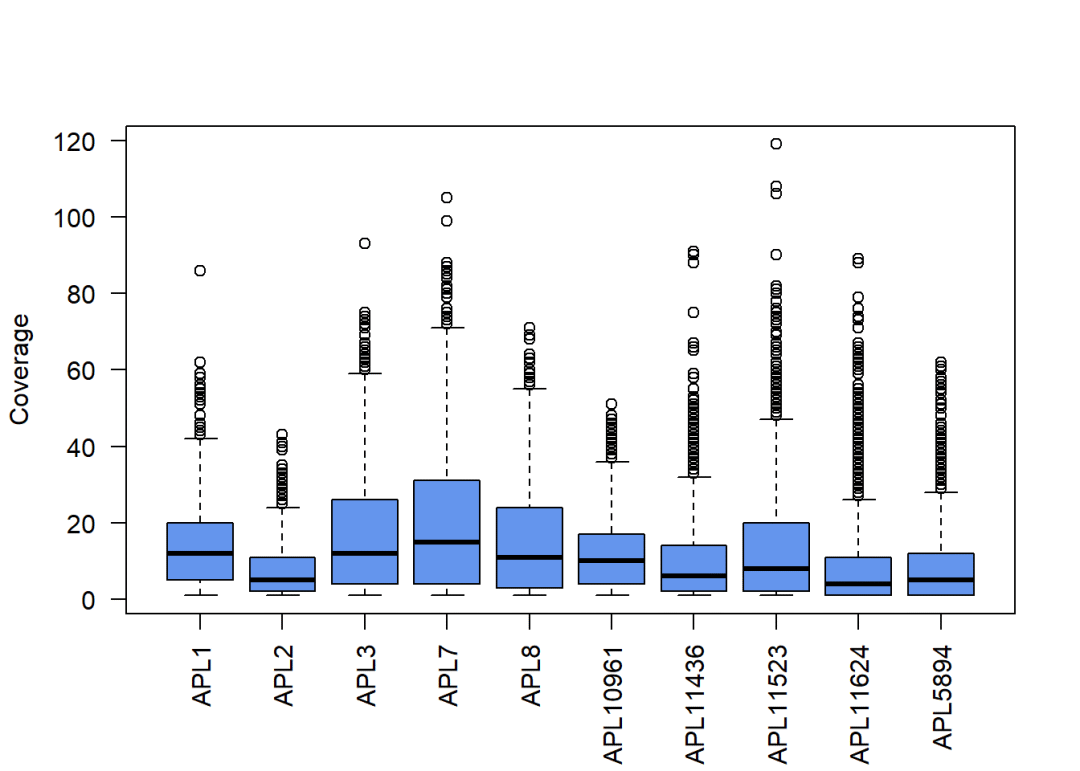

3.2 计算DMR

共分为五个步骤：

Definition of CpG clusters
Smooth methylation data within CpG clusters
Model and test group effect for each CpG site within CpG clusters
Apply hierarchical testing procedure: (a) Test CpG clusters for differential methylation and control weighted FDR on cluster (b) Trim rejected CpG clusters and control FDR on single CpGs
Define DMR boundaries

3.2.1 定义CpG cluster

复制代码

rrbs.small <- rrbs[1:1000,]#这里为了节省时间取了1000个基因出来运行，实际运行中这步不需要哦~
 rrbs.clust.unlim <-clusterSites(object = rrbs.small,
groups =colData(rrbs)$group,
perc.samples =4/5,
min.sites =20,
max.dist =100)

#这时每个CpG位点都会被聚类到所属的簇
head(rowRanges(rrbs.clust.unlim))

## GRanges object with 6 ranges and 1 metadata column:
##          seqnames    ranges strand |  cluster.id
##             <Rle> <IRanges>  <Rle> | <character>
##     1513     chr1    872335      * |      chr1_1
##     1514     chr1    872369      * |      chr1_1
##   401911     chr1    872370      * |      chr1_1
##     1515     chr1    872385      * |      chr1_1
##   401912     chr1    872386      * |      chr1_1
##     1516     chr1    872412      * |      chr1_1
##   -------
##   seqinfo: 25 sequences from an unspecified genome; no seqlengths

#cluster结果可以整合为一个GRanges对象：
clusterSitesToGR(rrbs.clust.unlim)

## GRanges object with 6 ranges and 1 metadata column:
##       seqnames        ranges strand |  cluster.id
##          <Rle>     <IRanges>  <Rle> | <character>
##   [1]     chr1 872335-872616      * |      chr1_1
##   [2]     chr1 875227-875470      * |      chr1_2
##   [3]     chr1 875650-876028      * |      chr1_3
##   [4]     chr1 876807-877458      * |      chr1_4
##   [5]     chr1 877684-877932      * |      chr1_5
##   [6]     chr2   45843-46937      * |      chr2_1
##   -------
##   seqinfo: 25 sequences from an unspecified genome; no seqlengths

3.2.2 Smooth methylation data

保留reads大于0的基因中的前90%

复制代码

ind.cov <-totalReads(rrbs.clust.unlim) >0
quant <-quantile(totalReads(rrbs.clust.unlim)[ind.cov], 0.9)
quant

## 90% 
##  32

rrbs.clust.lim <-limitCov(rrbs.clust.unlim, maxCov = quant)

默认以80bp的宽度对甲基化水平进行评分，这一步在LLinux中可以开启并行计算(Windows不支持)，当然，调用的核心数并不是越大越好：调用的线程越多就算的越快嘛?
Linux:

复制代码

predictedMeth <-predictMeth(object = rrbs.clust.lim,
mc.cores =6)

Windows:

复制代码

predictedMeth <-predictMeth(object = rrbs.clust.lim)

## 
  |                                                                            
  |                                                                      |   0%
  |                                                                            
  |=====================================================                 |  75%
  |                                                                            
  |======================================================================| 100%

predictedMeth#返回的是一个BSrel对象

## class: BSrel 
## dim: 344 10 
## metadata(0):
## assays(1): methLevel
## rownames(344): 1 2 ... 343 344
## rowData names(1): cluster.id
## colnames(10): APL1 APL2 ... APL11624 APL5894
## colData names(1): group

查看甲基化reads的覆盖度：

复制代码

covBoxplots(rrbs.clust.lim, col ="cornflowerblue", las =2)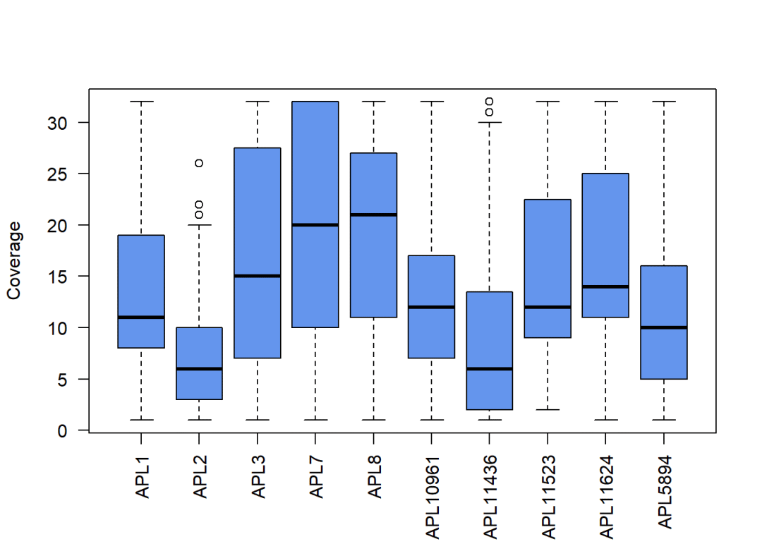

随序列位置变化甲基化程度曲线：

复制代码

plotMeth(object.raw = rrbs[,6],
object.rel = predictedMeth[,6],
region = region,
lwd.lines =2,
col.points ="blue",
cex =1.5)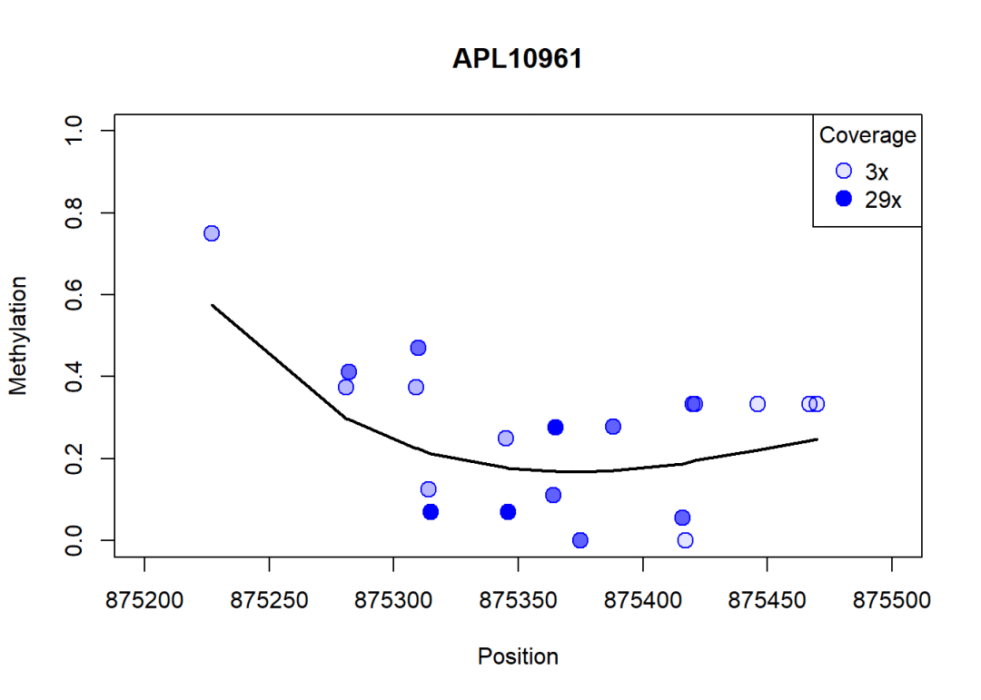

按照组别分开查看：

复制代码

#取出cancer与control两组：
cancer <- predictedMeth[, colData(predictedMeth)$group =="APL"]
control <- predictedMeth[, colData(predictedMeth)$group =="control"]
mean.cancer <-rowMeans(methLevel(cancer))
mean.control <-rowMeans(methLevel(control))
#可视化，看来这个区域中APLs的甲基化水平更高：
plot(mean.control,
mean.cancer,
col ="blue",
xlab ="Methylation in controls",
ylab ="Methylation in APLs")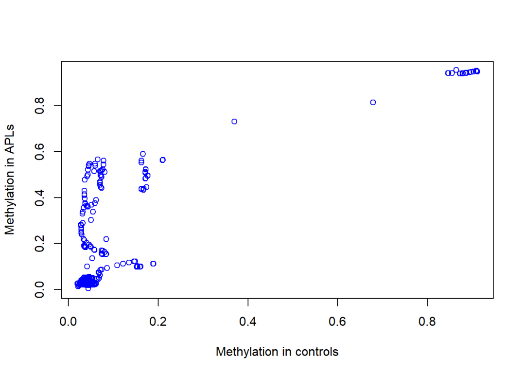

3.2.3 计算CpG位点组间差异

用beta regression来预测组间效应：

复制代码

betaResults <-betaRegression(formula =~group,
link ="probit",
object = predictedMeth,
type ="BR")
#生成的数据框记录了CpG位点的检验结果：
head(betaResults)

##      chr    pos        p.val meth.group1 meth.group2  meth.diff   estimate
## 1.1 chr1 872335 0.0011317652   0.9525098   0.8635983 0.08891149 -0.5730618
## 1.2 chr1 872369 0.0007678027   0.9414368   0.8444060 0.09703074 -0.5542171
## 1.3 chr1 872370 0.0008347451   0.9414314   0.8448725 0.09655890 -0.5522164
## 1.4 chr1 872385 0.0010337477   0.9412217   0.8521862 0.08903549 -0.5192564
## 1.5 chr1 872386 0.0010975571   0.9410544   0.8526863 0.08836810 -0.5156622
## 1.6 chr1 872412 0.0035114839   0.9378250   0.8718024 0.06602261 -0.4018161
##     std.error pseudo.R.sqrt cluster.id
## 1.1 0.1760266     0.6304051     chr1_1
## 1.2 0.1647422     0.6291904     chr1_1
## 1.3 0.1652843     0.6246474     chr1_1
## 1.4 0.1582531     0.6108452     chr1_1
## 1.5 0.1579728     0.6090794     chr1_1
## 1.6 0.1376551     0.5851744     chr1_1

3.2.4 计算CpG cluster差异

复制代码

#获得Z score的variogram：
vario.aux <-makeVariogram(betaResults)

|======================================================================| 100%

vario.aux包含两个list：

复制代码

names(vario.aux)

## [1] "variogram" "pValsList"

head(vario.aux$variogram[[1]])

##      h            v
## [1,] 1 0.0002565325
## [2,] 2 0.0014173211
## [3,] 3 0.0032763834
## [4,] 4 0.0044118674
## [5,] 5 0.0048485138
## [6,] 6 0.0089366555

head(vario.aux$pValsList[[1]])

##      chr    pos        p.val meth.group1 meth.group2  meth.diff   estimate
## 1.1 chr1 872335 0.0011317652   0.9525098   0.8635983 0.08891149 -0.5730618
## 1.2 chr1 872369 0.0007678027   0.9414368   0.8444060 0.09703074 -0.5542171
## 1.3 chr1 872370 0.0008347451   0.9414314   0.8448725 0.09655890 -0.5522164
## 1.4 chr1 872385 0.0010337477   0.9412217   0.8521862 0.08903549 -0.5192564
## 1.5 chr1 872386 0.0010975571   0.9410544   0.8526863 0.08836810 -0.5156622
## 1.6 chr1 872412 0.0035114839   0.9378250   0.8718024 0.06602261 -0.4018161
##     std.error pseudo.R.sqrt cluster.id  z.score pos.new
## 1.1 0.1760266     0.6304051     chr1_1 3.053282       1
## 1.2 0.1647422     0.6291904     chr1_1 3.167869      35
## 1.3 0.1652843     0.6246474     chr1_1 3.143485      36
## 1.4 0.1582531     0.6108452     chr1_1 3.080361      51
## 1.5 0.1579728     0.6090794     chr1_1 3.062480      52
## 1.6 0.1376551     0.5851744     chr1_1 2.695753      78

计算CpG cluster组间差异并矫正：

复制代码

vario.sm <-smoothVariogram(vario.aux, sill =0.9)
locCor <-estLocCor(vario.sm)
 clusters.rej <-testClusters(locCor,
FDR.cluster =0.1)

## 3 CpG clusters rejected.

移除显著差异的CpG cluster中不显著的CpG位点：

复制代码

clusters.trimmed <-trimClusters(clusters.rej,
FDR.loc =0.05)
head(clusters.trimmed)

##              chr    pos        p.val meth.group1 meth.group2  meth.diff
## chr1_1.1.1  chr1 872335 0.0011317652   0.9525098   0.8635983 0.08891149
## chr1_1.1.2  chr1 872369 0.0007678027   0.9414368   0.8444060 0.09703074
## chr1_1.1.3  chr1 872370 0.0008347451   0.9414314   0.8448725 0.09655890
## chr1_1.1.4  chr1 872385 0.0010337477   0.9412217   0.8521862 0.08903549
## chr1_1.1.5  chr1 872386 0.0010975571   0.9410544   0.8526863 0.08836810
## chr1_2.1.21 chr1 875227 0.0003916052   0.7175829   0.3648251 0.35275781
##               estimate std.error pseudo.R.sqrt cluster.id  z.score pos.new
## chr1_1.1.1  -0.5730618 0.1760266     0.6304051     chr1_1 3.053282       1
## chr1_1.1.2  -0.5542171 0.1647422     0.6291904     chr1_1 3.167869      35
## chr1_1.1.3  -0.5522164 0.1652843     0.6246474     chr1_1 3.143485      36
## chr1_1.1.4  -0.5192564 0.1582531     0.6108452     chr1_1 3.080361      51
## chr1_1.1.5  -0.5156622 0.1579728     0.6090794     chr1_1 3.062480      52
## chr1_2.1.21 -0.9212669 0.2598282     0.6818046     chr1_2 3.358661       1
##                    p.li
## chr1_1.1.1  0.015021790
## chr1_1.1.2  0.019813505
## chr1_1.1.3  0.021576860
## chr1_1.1.4  0.031691855
## chr1_1.1.5  0.033761681
## chr1_2.1.21 0.003649734

3.2.5 定义DMR边界

复制代码

DMRs <-findDMRs(clusters.trimmed,
max.dist =100,
diff.dir =TRUE)

## Warning in .merge_two_Seqinfo_objects(x, y): The 2 combined objects have no sequence levels in common. (Use
##   suppressWarnings() to suppress this warning.)

DMRs

## GRanges object with 4 ranges and 4 metadata columns:
##       seqnames        ranges strand |    median.p median.meth.group1
##          <Rle>     <IRanges>  <Rle> |   <numeric>          <numeric>
##   [1]     chr1 872335-872386      * | 1.03375e-03           0.941431
##   [2]     chr1 875227-875470      * | 6.67719e-06           0.502444
##   [3]     chr2   46126-46725      * | 5.23813e-05           0.432572
##   [4]     chr2   46915-46937      * | 1.48460e-02           0.136364
##       median.meth.group2 median.meth.diff
##                <numeric>        <numeric>
##   [1]          0.8521862        0.0890355
##   [2]          0.1820820        0.3194742
##   [3]          0.0769695        0.3528237
##   [4]          0.0369198        0.0994440
##   -------
##   seqinfo: 2 sequences from an unspecified genome; no seqlengths

3.2.6 两个样本间也可以计算DMR

就用上面的组间分析对象输入即可

复制代码

DMRs.2<-compareTwoSamples(object = predictedMeth,
sample1 ="APL1",
sample2 ="APL10961",
minDiff =0.3,
max.dist =100)
sum(overlapsAny(DMRs.2,DMRs))#可以如此取交集

## [1] 1

3.2.7 检测特定基因区域的甲基化差异

BiSeq内置方法：
不同的基因区域的甲基化水平差异经常对应着不同的生物学意义，例如启动子区域的甲基化往往会导致基因表达的抑制，而基因内部的甲基化水平差异可能会导致可变剪切的发生。
做法其实比较简单，先根据promoter的GRange提取BSraw对象的子集，再执行上面3.2计算DMR中的差异分析即可：

复制代码

data(promoters)
data(rrbs)
rrbs.red <-subsetByOverlaps(rrbs, promoters)
ov <-findOverlaps(rrbs.red, promoters)
rowRanges(rrbs.red)$cluster.id[queryHits(ov)] <- promoters$acc_no[subjectHits(ov)]
head(rowRanges(rrbs.red))

## GRanges object with 6 ranges and 1 metadata column:
##           seqnames    ranges strand |   cluster.id
##              <Rle> <IRanges>  <Rle> |  <character>
##   4636436     chr2     46089      + | NM_001077710
##   4636437     chr2     46095      + | NM_001077710
##   4636438     chr2     46104      + | NM_001077710
##   4636439     chr2     46111      + | NM_001077710
##   4636440     chr2     46113      + | NM_001077710
##   4636441     chr2     46126      + | NM_001077710
##   -------
##   seqinfo: 25 sequences from an unspecified genome; no seqlengths

#这里用rrbs.red得到的差异计算就仅包含promoters区域信息

调用globaltest进行计算：

复制代码

data(promoters)
data(rrbs)
rrbs <-rawToRel(rrbs)
promoters <- promoters[overlapsAny(promoters, rrbs)]
gt <-globalTest(group~1,
rrbs,
subsets = promoters)
head(gt)

##   p-value Statistic Expected Std.dev #Cov
## 1 0.00975  2.50e+01     11.1    4.89  206
## 2 0.05381  2.05e+01     11.1    5.61   67
## 3 0.05381  2.05e+01     11.1    5.61   67
## 4 1.00000  1.85e-31     11.1   14.81    8
## 5 1.00000  1.85e-31     11.1   14.81    8
## 6 0.06744  1.84e+01     11.1    4.88  149

3.3 下游数据处理

3.3.1 甲基化水平热图

这个矩阵的取值范围为0~1：

复制代码

 rowCols <-c("magenta", "blue")[as.numeric(colData(predictedMeth)$group)]

plotMethMap(predictedMeth,
region = DMRs[3],
groups =colData(predictedMeth)$group,
intervals =FALSE,
zlim =c(0,1),
RowSideColors = rowCols,
labCol ="", margins =c(0, 6))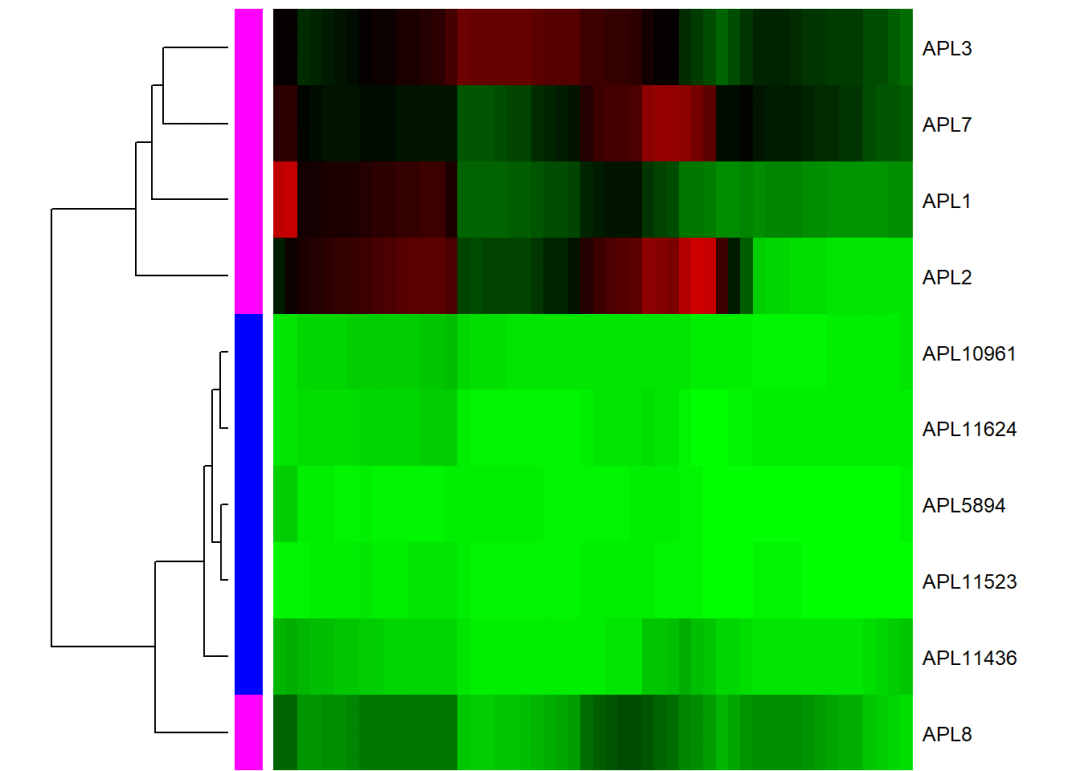

3.3.2 对比组间不同基因组位置甲基化水平：

复制代码

plotSmoothMeth(object.rel = predictedMeth,
region = DMRs[3],
groups =colData(predictedMeth)$group,
group.average =FALSE,
col =c("magenta", "blue"),
lwd =1.5)
legend("topright",
legend=levels(colData(predictedMeth)$group),
col=c("magenta", "blue"),
lty=1, lwd =1.5)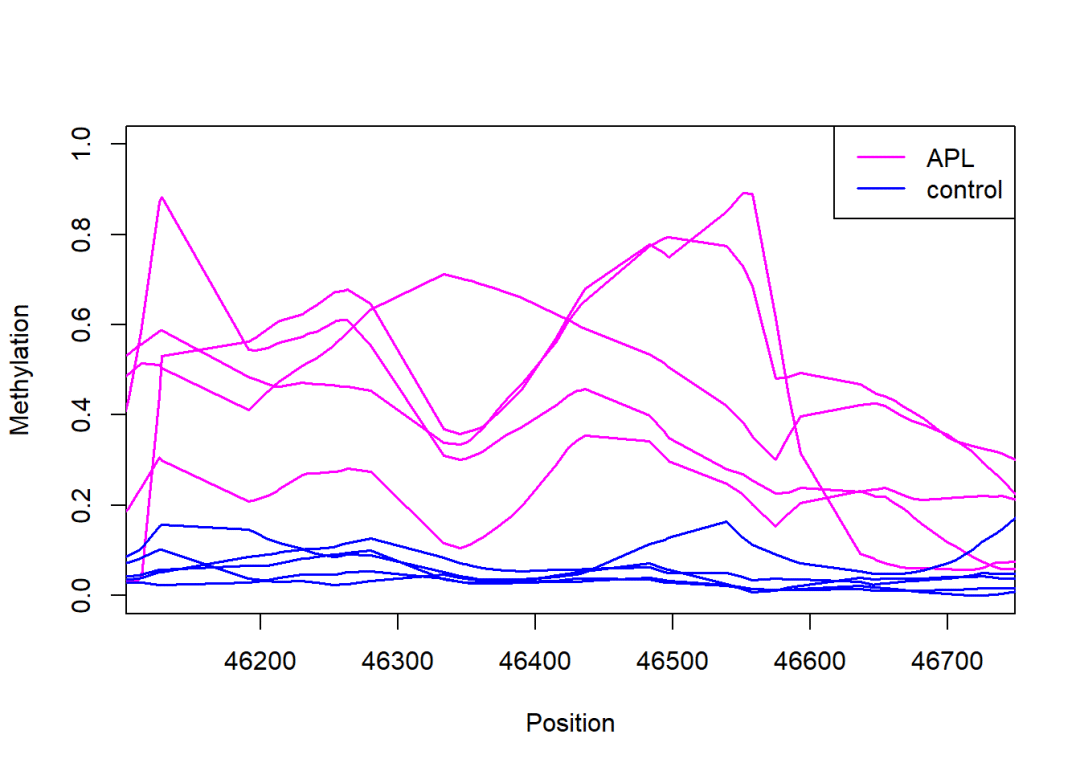

3.3.3 比对组间不同基因位置甲基化水平

还是以启动子举例：

复制代码

data(promoters)
head(promoters)

## GRanges object with 6 ranges and 1 metadata column:
##       seqnames            ranges strand |       acc_no
##          <Rle>         <IRanges>  <Rle> |  <character>
##   [1]     chr1 66998824-67000324      * |    NM_032291
##   [2]     chr1   8383389-8384889      * | NM_001080397
##   [3]     chr1 16766166-16767666      * | NM_001145277
##   [4]     chr1 16766166-16767666      * | NM_001145278
##   [5]     chr1 16766166-16767666      * |    NM_018090
##   [6]     chr1 50489126-50490626      * |    NM_032785
##   -------
##   seqinfo: 24 sequences from an unspecified genome; no seqlengths

#对DMR进行注释：  
DMRs.anno <-annotateGRanges(object = DMRs,
regions = promoters,
name ='Promoter',
regionInfo ='acc_no')
DMRs.anno

## GRanges object with 4 ranges and 5 metadata columns:
##       seqnames        ranges strand |    median.p median.meth.group1
##          <Rle>     <IRanges>  <Rle> |   <numeric>          <numeric>
##   [1]     chr1 872335-872386      * | 1.03375e-03           0.941431
##   [2]     chr1 875227-875470      * | 6.67719e-06           0.502444
##   [3]     chr2   46126-46725      * | 5.23813e-05           0.432572
##   [4]     chr2   46915-46937      * | 1.48460e-02           0.136364
##       median.meth.group2 median.meth.diff     Promoter
##                <numeric>        <numeric>  <character>
##   [1]          0.8521862        0.0890355         <NA>
##   [2]          0.1820820        0.3194742         <NA>
##   [3]          0.0769695        0.3528237 NM_001077710
##   [4]          0.0369198        0.0994440 NM_001077710
##   -------
##   seqinfo: 2 sequences from an unspecified genome; no seqlengths

#可视化：  
plotBindingSites(object = rrbs,
regions = promoters,
width =4000,#区域的宽度可以调整，0即为启动子起始位点
group =colData(rrbs)$group,
col =c("magenta", "blue"),
lwd =1.5)

|======================================================================| 100%

legend("top",
legend=levels(colData(rrbs)$group),
col=c("magenta", "blue"),
lty=1, lwd =1.5)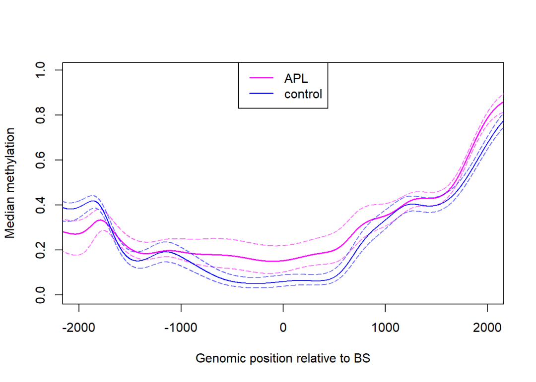

3.3.4 bed文件输出

bed文件可以用IGV浏览器进行可视化

复制代码

 track.names <-paste(colData(rrbs)$group,
"_",
gsub("APL", "", colnames(rrbs)),
sep="")
writeBED(object = rrbs,
name = track.names,
file =paste(colnames(rrbs), ".bed", sep =""))

## Warning in NSBS(i, x, exact = exact, strict.upper.bound = !allow.append, :
## subscript is an array, passing it thru as.vector() first

## Warning in NSBS(i, x, exact = exact, strict.upper.bound = !allow.append, :
## subscript is an array, passing it thru as.vector() first

## Warning in NSBS(i, x, exact = exact, strict.upper.bound = !allow.append, :
## subscript is an array, passing it thru as.vector() first

## Warning in NSBS(i, x, exact = exact, strict.upper.bound = !allow.append, :
## subscript is an array, passing it thru as.vector() first

## Warning in NSBS(i, x, exact = exact, strict.upper.bound = !allow.append, :
## subscript is an array, passing it thru as.vector() first

## Warning in NSBS(i, x, exact = exact, strict.upper.bound = !allow.append, :
## subscript is an array, passing it thru as.vector() first

## Warning in NSBS(i, x, exact = exact, strict.upper.bound = !allow.append, :
## subscript is an array, passing it thru as.vector() first

## Warning in NSBS(i, x, exact = exact, strict.upper.bound = !allow.append, :
## subscript is an array, passing it thru as.vector() first

## Warning in NSBS(i, x, exact = exact, strict.upper.bound = !allow.append, :
## subscript is an array, passing it thru as.vector() first

## Warning in NSBS(i, x, exact = exact, strict.upper.bound = !allow.append, :
## subscript is an array, passing it thru as.vector() first

## Warning in NSBS(i, x, exact = exact, strict.upper.bound = !allow.append, :
## subscript is an array, passing it thru as.vector() first

## Warning in NSBS(i, x, exact = exact, strict.upper.bound = !allow.append, :
## subscript is an array, passing it thru as.vector() first

## Warning in NSBS(i, x, exact = exact, strict.upper.bound = !allow.append, :
## subscript is an array, passing it thru as.vector() first

## Warning in NSBS(i, x, exact = exact, strict.upper.bound = !allow.append, :
## subscript is an array, passing it thru as.vector() first

## Warning in NSBS(i, x, exact = exact, strict.upper.bound = !allow.append, :
## subscript is an array, passing it thru as.vector() first

## Warning in NSBS(i, x, exact = exact, strict.upper.bound = !allow.append, :
## subscript is an array, passing it thru as.vector() first

## Warning in NSBS(i, x, exact = exact, strict.upper.bound = !allow.append, :
## subscript is an array, passing it thru as.vector() first

## Warning in NSBS(i, x, exact = exact, strict.upper.bound = !allow.append, :
## subscript is an array, passing it thru as.vector() first

## Warning in NSBS(i, x, exact = exact, strict.upper.bound = !allow.append, :
## subscript is an array, passing it thru as.vector() first

## Warning in NSBS(i, x, exact = exact, strict.upper.bound = !allow.append, :
## subscript is an array, passing it thru as.vector() first

writeBED(object = predictedMeth,
name = track.names,
file =paste(colnames(predictedMeth), ".bed", sep =""))

## Warning in NSBS(i, x, exact = exact, strict.upper.bound = !allow.append, :
## subscript is an array, passing it thru as.vector() first

## Warning in NSBS(i, x, exact = exact, strict.upper.bound = !allow.append, :
## subscript is an array, passing it thru as.vector() first

## Warning in NSBS(i, x, exact = exact, strict.upper.bound = !allow.append, :
## subscript is an array, passing it thru as.vector() first

## Warning in NSBS(i, x, exact = exact, strict.upper.bound = !allow.append, :
## subscript is an array, passing it thru as.vector() first

## Warning in NSBS(i, x, exact = exact, strict.upper.bound = !allow.append, :
## subscript is an array, passing it thru as.vector() first

## Warning in NSBS(i, x, exact = exact, strict.upper.bound = !allow.append, :
## subscript is an array, passing it thru as.vector() first

## Warning in NSBS(i, x, exact = exact, strict.upper.bound = !allow.append, :
## subscript is an array, passing it thru as.vector() first

## Warning in NSBS(i, x, exact = exact, strict.upper.bound = !allow.append, :
## subscript is an array, passing it thru as.vector() first

## Warning in NSBS(i, x, exact = exact, strict.upper.bound = !allow.append, :
## subscript is an array, passing it thru as.vector() first

## Warning in NSBS(i, x, exact = exact, strict.upper.bound = !allow.append, :
## subscript is an array, passing it thru as.vector() first

## Warning in NSBS(i, x, exact = exact, strict.upper.bound = !allow.append, :
## subscript is an array, passing it thru as.vector() first

## Warning in NSBS(i, x, exact = exact, strict.upper.bound = !allow.append, :
## subscript is an array, passing it thru as.vector() first

## Warning in NSBS(i, x, exact = exact, strict.upper.bound = !allow.append, :
## subscript is an array, passing it thru as.vector() first

## Warning in NSBS(i, x, exact = exact, strict.upper.bound = !allow.append, :
## subscript is an array, passing it thru as.vector() first

## Warning in NSBS(i, x, exact = exact, strict.upper.bound = !allow.append, :
## subscript is an array, passing it thru as.vector() first

## Warning in NSBS(i, x, exact = exact, strict.upper.bound = !allow.append, :
## subscript is an array, passing it thru as.vector() first

## Warning in NSBS(i, x, exact = exact, strict.upper.bound = !allow.append, :
## subscript is an array, passing it thru as.vector() first

## Warning in NSBS(i, x, exact = exact, strict.upper.bound = !allow.append, :
## subscript is an array, passing it thru as.vector() first

## Warning in NSBS(i, x, exact = exact, strict.upper.bound = !allow.append, :
## subscript is an array, passing it thru as.vector() first

## Warning in NSBS(i, x, exact = exact, strict.upper.bound = !allow.append, :
## subscript is an array, passing it thru as.vector() first

四、找个测试文件试试

上面的教学比较详细，不够流畅，我们找两个文件自己试试：

复制代码

list.files('测试数据/')
wgbs1 <-readBismark('测试数据/Sample1.deduplicated.bismark.cov.gz',
colData=DataFrame(sample="sample1",group='group_A'))
wgbs2 <-readBismark('测试数据/Sample2.deduplicated.bismark.cov.gz',
colData=DataFrame(sample="sample2",group='group_B'))
wgbs3 <-readBismark('测试数据/Sample3.deduplicated.bismark.cov.gz',
colData=DataFrame(sample="sample3",group='group_B'))
mywgbs <-combine(wgbs1,wgbs2,wgbs3)
mywgbs
mywgbs <-rawToRel(mywgbs)
covStatistics(mywgbs)
covBoxplots(mywgbs, col ="cornflowerblue", las =2)#绘图

mywgbs@colData$group <-factor(mywgbs@colData$group,levels =c('group_A','group_B'))

mywgbs <-clusterSites(object = mywgbs,
groups =colData(mywgbs)$group,
perc.samples =1/3,#大于多少即在所有样本中该位点的覆盖比例要高于这个值，0即为不过滤
min.sites =20,
max.dist =100)

五、引用是美德

复制代码

Katja Hebestreit, Martin Dugas, and Hans-Ulrich Klein. Detection of
significantly differentially methylated regions in targeted bisulfite sequencing data. Bioinformatics, 29(13):1647--1653, Jul 2013. URL:
http://dx.doi.org/10.1093/bioinformatics/btt263,
doi:10.1093/bioinformatics/btt263

六、欢迎致谢

复制代码

Since Biomamba and his wechat public account team produce bioinformatics tutorials elaborately and share code with annotation, we thank Biomamba for their guidance in bioinformatics and data analysis for the current study.

Biseq计算差异甲基化区域

一、写在前面

二、数据输入

2.1 BSraw

2.1.1 快速创建输入数据：

2.1.2 手动创建输入数据

2.1.3 测试数据：

2.2 BSrel

2.2.1 手动创建：

2.3 BiSeq对象简单处理

三、数据分析

3.1 质控

3.2 计算DMR

3.2.1 定义CpG cluster

3.2.2 Smooth methylation data

3.2.3 计算CpG位点组间差异

3.2.4 计算CpG cluster差异

3.2.5 定义DMR边界

3.2.6 两个样本间也可以计算DMR

3.2.7 检测特定基因区域的甲基化差异

3.3 下游数据处理

3.3.1 甲基化水平热图

3.3.2 对比组间不同基因组位置甲基化水平：

3.3.3 比对组间不同基因位置甲基化水平

3.3.4 bed文件输出

四、找个测试文件试试

五、引用是美德

六、欢迎致谢

2.1 `BSraw`

2.2 `BSrel`

2.3 `BiSeq`对象简单处理