π的十种数值计算方法

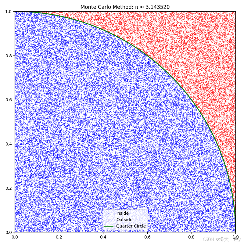
1. 蒙特卡洛方法 (Monte Carlo)

原理：在单位正方形内随机撒点，计算落在1/4圆内的比例。

import numpy as np
import matplotlib.pyplot as plt

def monte_carlo_pi(n_samples=10000):
    x = np.random.uniform(0, 1, n_samples)
    y = np.random.uniform(0, 1, n_samples)
    inside = (x**2 + y**2) <= 1
    pi_est = 4 * np.sum(inside) / n_samples
    
    # 可视化
    fig, ax = plt.subplots(figsize=(8, 8))
    ax.scatter(x[inside], y[inside], c='blue', s=1, alpha=0.5, label='Inside')
    ax.scatter(x[~inside], y[~inside], c='red', s=1, alpha=0.5, label='Outside')
    
    theta = np.linspace(0, np.pi/2, 100)
    ax.plot(np.cos(theta), np.sin(theta), 'g-', linewidth=2, label='Quarter Circle')
    ax.set_xlim(0, 1)
    ax.set_ylim(0, 1)
    ax.set_aspect('equal')
    ax.legend()
    ax.set_title(f'Monte Carlo Method: π ≈ {pi_est:.6f}')
    plt.tight_layout()
    plt.show()
    plt.savefig('pi_est.png')
    return pi_est

print(f"蒙特卡洛方法: π ≈ {monte_carlo_pi(50000):.10f}")

🍎运行结果：

蒙特卡洛方法: π ≈ 3.1435200000

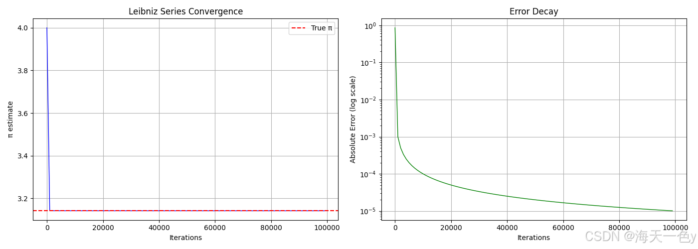
2. 莱布尼茨级数 (Leibniz Series)

原理：π/4 = 1 - 1/3 + 1/5 - 1/7 + 1/9 - ...

import numpy as np
import matplotlib.pyplot as plt
def leibniz_pi(n_terms=100000):
    pi_est = 0
    history = []
    for k in range(n_terms):
        term = ((-1)**k) / (2*k + 1)
        pi_est += term
        if k % 1000 == 0:
            history.append(4 * pi_est)
    
    pi_est *= 4
    
    # 可视化收敛过程
    fig, (ax1, ax2) = plt.subplots(1, 2, figsize=(14, 5))
    
    # 收敛曲线
    iterations = np.arange(0, n_terms, 1000)
    ax1.plot(iterations, history, 'b-', linewidth=1)
    ax1.axhline(y=np.pi, color='r', linestyle='--', label='True π')
    ax1.set_xlabel('Iterations')
    ax1.set_ylabel('π estimate')
    ax1.set_title('Leibniz Series Convergence')
    ax1.legend()
    ax1.grid(True)
    
    # 误差分析
    errors = [abs(h - np.pi) for h in history]
    ax2.semilogy(iterations, errors, 'g-', linewidth=1)
    ax2.set_xlabel('Iterations')
    ax2.set_ylabel('Absolute Error (log scale)')
    ax2.set_title('Error Decay')
    ax2.grid(True)
    
    plt.tight_layout()
    plt.show()
    plt.savefig('leibniz_convergence.png')
    
    return pi_est

print(f"莱布尼茨级数: π ≈ {leibniz_pi(100000):.10f}")

🍎运行结果：

(langchain) root@dsw-1656158-555c7989dd-wb77c:/mnt/workspace/pi# python demo2.py

莱布尼茨级数: π ≈ 3.1415826536

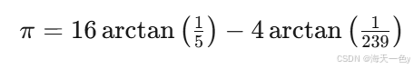
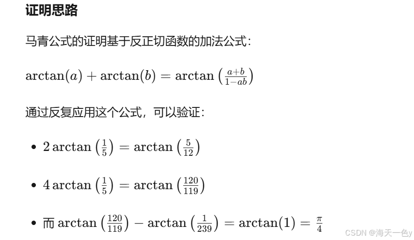
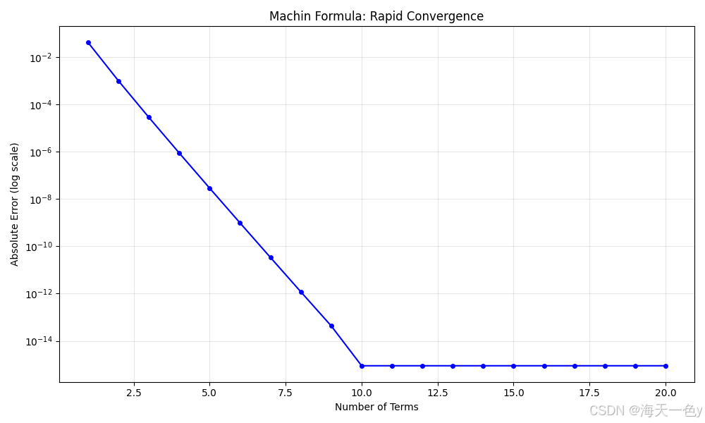
3. 马青公式 (Machin Formula)

原理：π/4 = 4·arctan(1/5) - arctan(1/239)，利用arctan的泰勒展开。

马青公式（Machin Formula）是计算圆周率 π 的经典公式之一，由英国天文学家约翰·马青（John Machin）于1706年发现。这个公式在数学史上具有重要意义，因为它使得人类首次将 π 计算到了100位小数。

公式表达式

马青公式的形式为：

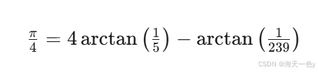
或者等价地写成：

🍊代码实现：

import numpy as np
import matplotlib.pyplot as plt

def arctan_series(x, n_terms=50):
    """计算arctan(x)的泰勒级数"""
    result = 0
    for n in range(n_terms):
        term = ((-1)**n) * (x**(2*n + 1)) / (2*n + 1)
        result += term
    return result

def machin_pi(n_terms=50):
    # π/4 = 4*arctan(1/5) - arctan(1/239)
    pi_est = 4 * (4 * arctan_series(1/5, n_terms) - arctan_series(1/239, n_terms))
    
    # 可视化不同项数的精度
    terms_range = range(1, n_terms + 1)
    estimates = []
    for n in terms_range:
        est = 4 * (4 * arctan_series(1/5, n) - arctan_series(1/239, n))
        estimates.append(est)
    
    errors = [abs(e - np.pi) for e in estimates]
    
    plt.figure(figsize=(10, 6))
    plt.semilogy(terms_range, errors, 'bo-', markersize=4)
    plt.xlabel('Number of Terms')
    plt.ylabel('Absolute Error (log scale)')
    plt.title('Machin Formula: Rapid Convergence')
    plt.grid(True, alpha=0.3)
    plt.tight_layout()
    # plt.show()
    plt.savefig('machin_convergence.png')
    return pi_est

print(f"马青公式: π ≈ {machin_pi(20):.15f}")

🍎运行结果：

(langchain) root@dsw-1656158-555c7989dd-wb77c:/mnt/workspace/pi# python demo3.py

马青公式: π ≈ 3.141592653589794

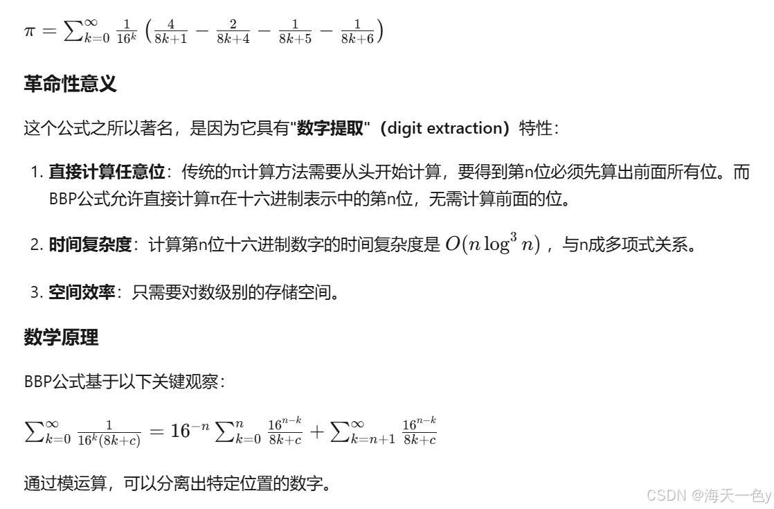
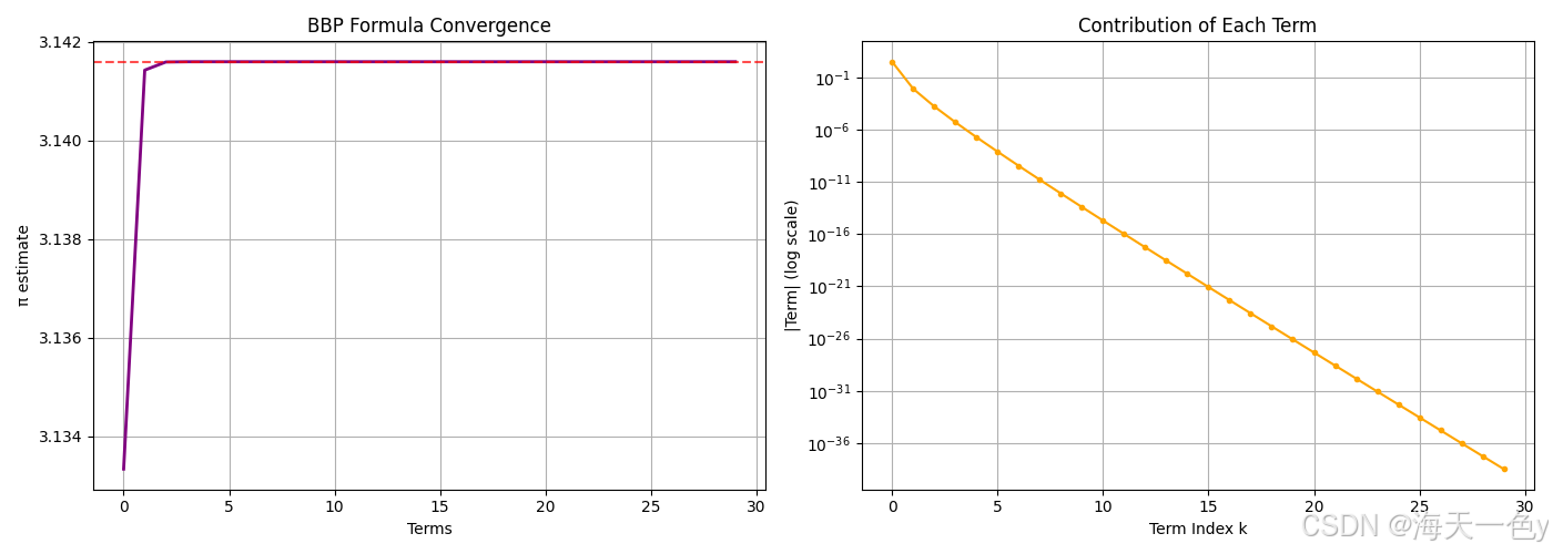
4. 贝利-波尔温-普劳夫公式 (BBP Formula)

原理：可直接计算π的第n位十六进制，无需计算前面各位。

BBP公式是1995年由三位数学家大卫·贝利（David Bailey） 、彼得·波尔温（Peter Borwein） 和**西蒙·普劳夫（Simon Plouffe）**共同发现的，用于计算π的十六进制（十六进制）展开的公式。

公式表达式

import numpy as np
import matplotlib.pyplot as plt

def bbp_pi(n_terms=50):
    """BBP公式: π = Σ (1/16^k) * (4/(8k+1) - 2/(8k+4) - 1/(8k+5) - 1/(8k+6))"""
    pi_est = 0
    history = []
    
    for k in range(n_terms):
        term = (1/(16**k)) * (4/(8*k+1) - 2/(8*k+4) - 1/(8*k+5) - 1/(8*k+6))
        pi_est += term
        history.append(pi_est)
    
    # 可视化
    fig, (ax1, ax2) = plt.subplots(1, 2, figsize=(14, 5))
    
    # 收敛速度
    ax1.plot(range(n_terms), history, 'purple', linewidth=2)
    ax1.axhline(y=np.pi, color='r', linestyle='--', alpha=0.7)
    ax1.set_xlabel('Terms')
    ax1.set_ylabel('π estimate')
    ax1.set_title('BBP Formula Convergence')
    ax1.grid(True)
    
    # 每项的贡献（对数尺度）
    contributions = []
    for k in range(n_terms):
        contrib = abs((1/(16**k)) * (4/(8*k+1) - 2/(8*k+4) - 1/(8*k+5) - 1/(8*k+6)))
        contributions.append(contrib)
    
    ax2.semilogy(range(n_terms), contributions, 'orange', marker='o', markersize=3)
    ax2.set_xlabel('Term Index k')
    ax2.set_ylabel('|Term| (log scale)')
    ax2.set_title('Contribution of Each Term')
    ax2.grid(True)
    
    plt.tight_layout()
    plt.show()
    plt.savefig('bbp_convergence.png')
    
    return pi_est

print(f"BBP公式: π ≈ {bbp_pi(30):.15f}")

🍎运行结果：

(langchain) root@dsw-1656158-555c7989dd-wb77c:/mnt/workspace/pi# python demo4.py

BBP公式: π ≈ 3.141592653589793

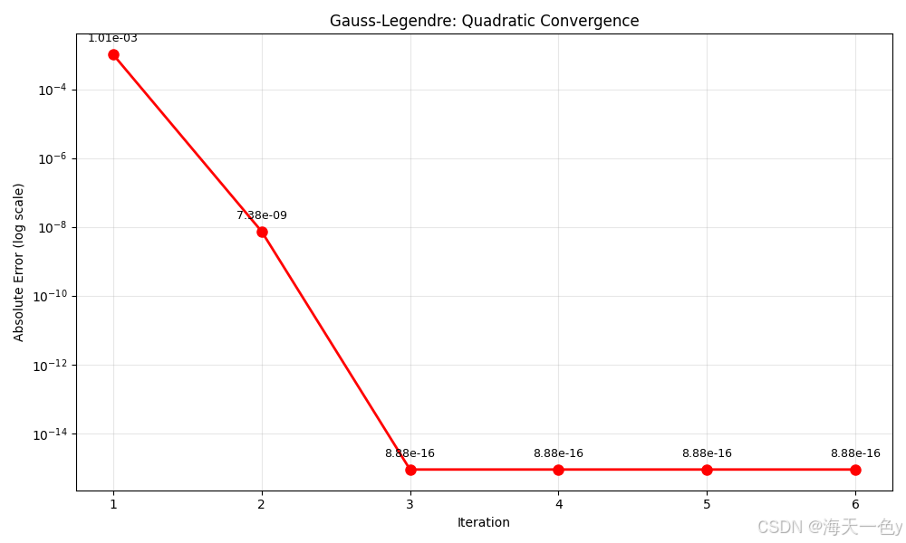
5. 高斯-勒让德算法 (Gauss-Legendre)

原理：迭代算法，每次迭代精度翻倍，是已知收敛最快的算法之一。

import numpy as np
import matplotlib.pyplot as plt

def gauss_legendre_pi(iterations=5):
    """高斯-勒让德算法，二次收敛"""
    a = 1.0
    b = 1/np.sqrt(2)
    t = 1/4
    p = 1.0
    
    history = []
    
    for i in range(iterations):
        a_next = (a + b) / 2
        b = np.sqrt(a * b)
        t -= p * (a - a_next)**2
        p *= 2
        a = a_next
        
        pi_est = (a + b)**2 / (4 * t)
        history.append(pi_est)
        print(f"Iteration {i+1}: π ≈ {pi_est:.15f}")
    
    # 可视化
    plt.figure(figsize=(10, 6))
    iterations_range = range(1, iterations + 1)
    errors = [abs(h - np.pi) for h in history]
    
    plt.semilogy(iterations_range, errors, 'ro-', markersize=8, linewidth=2)
    plt.xlabel('Iteration')
    plt.ylabel('Absolute Error (log scale)')
    plt.title('Gauss-Legendre: Quadratic Convergence')
    plt.grid(True, alpha=0.3)
    
    # 添加精度翻倍标注
    for i, err in enumerate(errors):
        plt.annotate(f'{err:.2e}', (i+1, err), textcoords="offset points", 
                    xytext=(0,10), ha='center', fontsize=9)
    
    plt.tight_layout()
    plt.show()
    plt.savefig('gauss_legendre_convergence.png')
    return history[-1]

print(f"\n高斯-勒让德算法: π ≈ {gauss_legendre_pi(6):.15f}")

🍎运行结果：

(langchain) root@dsw-1656158-555c7989dd-wb77c:/mnt/workspace/pi# python demo5.py

Iteration 1: π ≈ 3.140579250522169

Iteration 2: π ≈ 3.141592646213543

Iteration 3: π ≈ 3.141592653589794

Iteration 4: π ≈ 3.141592653589794

Iteration 5: π ≈ 3.141592653589794

Iteration 6: π ≈ 3.141592653589794

高斯-勒让德算法: π ≈ 3.141592653589794

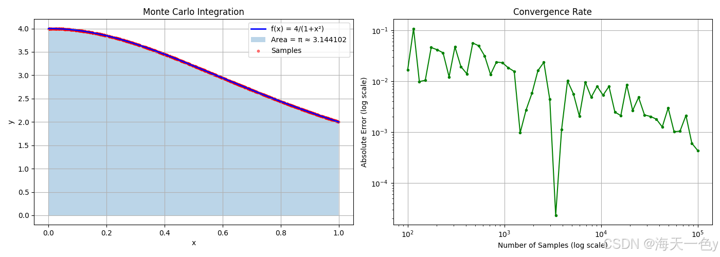
6. 蒙特卡洛积分法 (Integration)

原理：利用∫₀¹ 4/(1+x²) dx = π。

🍊代码实现：

import numpy as np
import matplotlib.pyplot as plt

def monte_carlo_integration_pi(n_samples=100000):
    """计算∫₀¹ 4/(1+x²) dx = π"""
    x = np.random.uniform(0, 1, n_samples)
    y = 4 / (1 + x**2)
    pi_est = np.mean(y)
    
    # 可视化积分区域
    fig, (ax1, ax2) = plt.subplots(1, 2, figsize=(14, 5))
    
    # 函数图像和采样点
    x_fine = np.linspace(0, 1, 1000)
    y_fine = 4 / (1 + x_fine**2)
    
    ax1.plot(x_fine, y_fine, 'b-', linewidth=2, label='f(x) = 4/(1+x²)')
    ax1.fill_between(x_fine, 0, y_fine, alpha=0.3, label=f'Area = π ≈ {pi_est:.6f}')
    ax1.scatter(x[::100], y[::100], c='red', s=10, alpha=0.5, label='Samples')
    ax1.set_xlabel('x')
    ax1.set_ylabel('y')
    ax1.legend()
    ax1.set_title('Monte Carlo Integration')
    ax1.grid(True)
    
    # 收敛分析
    sample_sizes = np.logspace(2, 5, 50, dtype=int)
    estimates = []
    for n in sample_sizes:
        x_temp = np.random.uniform(0, 1, n)
        y_temp = 4 / (1 + x_temp**2)
        estimates.append(np.mean(y_temp))
    
    errors = [abs(e - np.pi) for e in estimates]
    ax2.loglog(sample_sizes, errors, 'g-', marker='o', markersize=3)
    ax2.set_xlabel('Number of Samples (log scale)')
    ax2.set_ylabel('Absolute Error (log scale)')
    ax2.set_title('Convergence Rate')
    ax2.grid(True)
    
    plt.tight_layout()
    plt.show()
    plt.savefig('monte_carlo_integration_pi.png')
    
    return pi_est

print(f"蒙特卡洛积分: π ≈ {monte_carlo_integration_pi(100000):.10f}")

🍎运行结果：

(langchain) root@dsw-1656158-555c7989dd-wb77c:/mnt/workspace/pi# python demo6.py

蒙特卡洛积分: π ≈ 3.1441017045

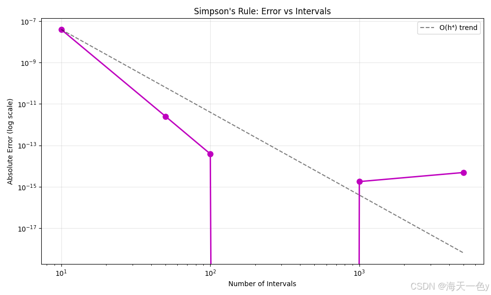
7. 辛普森数值积分 (Simpson's Rule)

原理：用抛物线近似函数曲线进行数值积分。

🍊代码实现：

import numpy as np
import matplotlib.pyplot as plt

def simpson_pi(n_intervals=1000):
    """使用辛普森法则计算∫₀¹ 4/(1+x²) dx"""
    def f(x):
        return 4 / (1 + x**2)
    
    a, b = 0, 1
    h = (b - a) / n_intervals
    
    # 辛普森法则: (h/3) * [f(x₀) + 4Σf(x_odd) + 2Σf(x_even) + f(xₙ)]
    result = f(a) + f(b)
    
    for i in range(1, n_intervals):
        x = a + i * h
        if i % 2 == 0:
            result += 2 * f(x)
        else:
            result += 4 * f(x)
    
    pi_est = result * h / 3
    
    # 可视化不同区间数的效果
    intervals = [10, 50, 100, 500, 1000, 5000]
    errors = []
    
    for n in intervals:
        h_temp = (b - a) / n
        res = f(a) + f(b)
        for i in range(1, n):
            x = a + i * h_temp
            coef = 4 if i % 2 == 1 else 2
            res += coef * f(x)
        pi_temp = res * h_temp / 3
        errors.append(abs(pi_temp - np.pi))
    
    plt.figure(figsize=(10, 6))
    plt.loglog(intervals, errors, 'mo-', markersize=8, linewidth=2)
    plt.xlabel('Number of Intervals')
    plt.ylabel('Absolute Error (log scale)')
    plt.title("Simpson's Rule: Error vs Intervals")
    plt.grid(True, alpha=0.3)
    
    # 添加趋势线（辛普森误差应为O(h⁴)）
    x_trend = np.array(intervals)
    y_trend = errors[0] * (intervals[0]/x_trend)**4
    plt.loglog(x_trend, y_trend, 'k--', alpha=0.5, label='O(h⁴) trend')
    plt.legend()
    
    plt.tight_layout()
    plt.show()
    plt.savefig('simpson_error.png')
    
    return pi_est

print(f"辛普森积分: π ≈ {simpson_pi(10000):.12f}")

🍎运行结果：

(langchain) root@dsw-1656158-555c7989dd-wb77c:/mnt/workspace/pi# python demo7.py

辛普森积分: π ≈ 3.141592653590

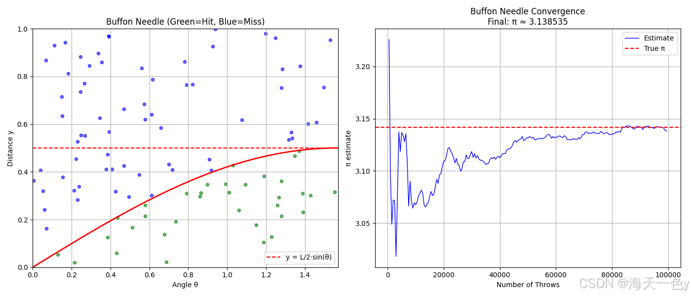
8. 布丰投针问题 (Buffon's Needle)

原理：随机投针，根据针与平行线相交的概率估计π。

🍊实现代码：

import numpy as np
import matplotlib.pyplot as plt

def buffon_needle_pi(n_throws=50000, needle_length=1.0, line_spacing=2.0):
    """布丰投针实验"""
    if needle_length > line_spacing:
        raise ValueError("Needle length should be <= line spacing")
    
    hits = 0
    history = []
    
    for i in range(n_throws):
        # 随机位置：针中心到最近线的距离
        y = np.random.uniform(0, line_spacing/2)
        # 随机角度
        theta = np.random.uniform(0, np.pi/2)
        
        # 如果针与线相交
        if y <= (needle_length/2) * np.sin(theta):
            hits += 1
        
        # 记录历史
        if i > 0 and i % 500 == 0:
            if hits > 0:
                pi_est = (2 * needle_length * i) / (line_spacing * hits)
                history.append((i, pi_est))
    
    pi_est = (2 * needle_length * n_throws) / (line_spacing * hits) if hits > 0 else 0
    
    # 可视化
    fig, (ax1, ax2) = plt.subplots(1, 2, figsize=(14, 6))
    
    # 模拟可视化（部分投针）
    n_display = 100
    ax1.set_xlim(0, np.pi/2)
    ax1.set_ylim(0, line_spacing/2)
    ax1.axhline(y=needle_length/2, color='r', linestyle='--', label='y = L/2·sin(θ)')
    
    theta_range = np.linspace(0, np.pi/2, 100)
    ax1.plot(theta_range, (needle_length/2)*np.sin(theta_range), 'r-', linewidth=2)
    
    # 绘制一些随机点
    for _ in range(n_display):
        y = np.random.uniform(0, line_spacing/2)
        theta = np.random.uniform(0, np.pi/2)
        color = 'green' if y <= (needle_length/2)*np.sin(theta) else 'blue'
        ax1.scatter(theta, y, c=color, s=20, alpha=0.6)
    
    ax1.set_xlabel('Angle θ')
    ax1.set_ylabel('Distance y')
    ax1.set_title(f'Buffon Needle (Green=Hit, Blue=Miss)')
    ax1.legend()
    ax1.grid(True)
    
    # 收敛曲线
    if history:
        throws, estimates = zip(*history)
        ax2.plot(throws, estimates, 'b-', linewidth=1, label='Estimate')
        ax2.axhline(y=np.pi, color='r', linestyle='--', label='True π')
        ax2.set_xlabel('Number of Throws')
        ax2.set_ylabel('π estimate')
        ax2.set_title(f'Buffon Needle Convergence\nFinal: π ≈ {pi_est:.6f}')
        ax2.legend()
        ax2.grid(True)
    
    plt.tight_layout()
    plt.show()
    plt.savefig('buffon_needle.png')
    
    return pi_est

print(f"布丰投针: π ≈ {buffon_needle_pi(100000):.10f}")

🍎运行结果：

(langchain) root@dsw-1656158-555c7989dd-wb77c:/mnt/workspace/pi# python demo8.py

布丰投针: π ≈ 3.1385349319

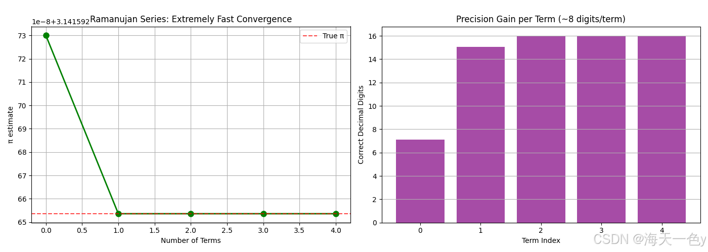
9. 拉马努金公式 (Ramanujan Series)

原理：收敛极快的级数，每增加一项可获得约8位小数精度。

🍊实现代码：

import numpy as np
import matplotlib.pyplot as plt
import math  # 添加标准库 math 模块

def ramanujan_pi(n_terms=10):
    """拉马努金公式: 1/π = (2√2/9801) * Σ (4k)!(1103+26390k)/((k!)⁴ 396⁴ᵏ)"""
    sum_val = 0
    history = []
    
    for k in range(n_terms):
        # 使用 math.factorial 替代 np.math.factorial
        numerator = math.factorial(4*k) * (1103 + 26390*k)
        denominator = (math.factorial(k)**4) * (396**(4*k))
        term = numerator / denominator
        sum_val += term
        
        pi_est = 9801 / (2 * np.sqrt(2) * sum_val)
        history.append(pi_est)
        print(f"Term {k}: π ≈ {pi_est:.15f}")
    
    # 可视化惊人的收敛速度
    fig, (ax1, ax2) = plt.subplots(1, 2, figsize=(14, 5))
    
    # 估计值快速收敛
    ax1.plot(range(n_terms), history, 'go-', markersize=8, linewidth=2)
    ax1.axhline(y=np.pi, color='r', linestyle='--', alpha=0.7, label='True π')
    ax1.set_xlabel('Number of Terms')
    ax1.set_ylabel('π estimate')
    ax1.set_title('Ramanujan Series: Extremely Fast Convergence')
    ax1.legend()
    ax1.grid(True)
    
    # 精度位数
    precision_digits = [-np.log10(abs(h - np.pi)) if h != np.pi else 16 for h in history]
    ax2.bar(range(n_terms), precision_digits, color='purple', alpha=0.7)
    ax2.set_xlabel('Term Index')
    ax2.set_ylabel('Correct Decimal Digits')
    ax2.set_title('Precision Gain per Term (~8 digits/term)')
    ax2.grid(True, axis='y')
    
    plt.tight_layout()
    plt.show()
    plt.savefig('ramanujan_series.png')
    return history[-1]

print(f"\n拉马努金公式: π ≈ {ramanujan_pi(5):.15f}")

🍎运行结果：

(langchain) root@dsw-1656158-555c7989dd-wb77c:/mnt/workspace/pi# python demo9.py

Term 0: π ≈ 3.141592730013306

Term 1: π ≈ 3.141592653589794

Term 2: π ≈ 3.141592653589793

Term 3: π ≈ 3.141592653589793

Term 4: π ≈ 3.141592653589793

拉马努金公式: π ≈ 3.141592653589793

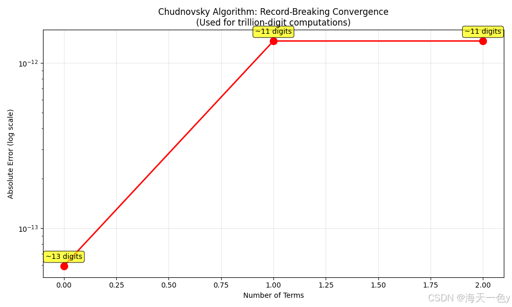
10. 楚德诺夫斯基算法 (Chudnovsky Algorithm)

原理：拉马努金公式的改进版，收敛更快，曾用于计算π的万亿位。

🍊实现代码：

import numpy as np
import matplotlib.pyplot as plt
import math

def chudnovsky_pi(n_terms=3):
    """楚德诺夫斯基算法: 1/π = 12 * Σ (-1)ᵏ (6k)! (13591409 + 545140134k) / ((3k)!(k!)³ 640320³ᵏ⁺³/²)"""
    sum_val = 0
    history = []
    
    C = 640320
    C3_over_24 = C**3 / 24
    
    for k in range(n_terms):
        numerator = ((-1)**k) * math.factorial(6*k) * (13591409 + 545140134*k)
        denominator = (math.factorial(3*k) * (math.factorial(k)**3)) * (C3_over_24**k)
        sum_val += numerator / denominator
        
        pi_est = 426880 * np.sqrt(10005) / sum_val
        history.append(pi_est)
        print(f"Term {k}: π ≈ {pi_est:.20f}")
    
    # 可视化
    fig, ax = plt.subplots(figsize=(10, 6))
    
    errors = [abs(h - np.pi) for h in history]
    iterations = range(n_terms)
    
    # 修复：移除重复的 markersize12 参数
    ax.semilogy(iterations, errors, 'ro-', markersize=10, linewidth=2)
    ax.set_xlabel('Number of Terms')
    ax.set_ylabel('Absolute Error (log scale)')
    ax.set_title('Chudnovsky Algorithm: Record-Breaking Convergence\n(Used for trillion-digit computations)')
    ax.grid(True, alpha=0.3)
    
    # 修复：处理 error 为 0 的情况（当 k=0 时可能完全精确）
    for i, err in enumerate(errors):
        if err > 0:
            digits = int(-np.log10(err))
        else:
            digits = 30  # 如果误差为0，假设极高精度
        ax.annotate(f'~{digits} digits', (i, err if err > 0 else 1e-30), 
                   textcoords="offset points", 
                   xytext=(0, 10), ha='center', fontsize=10, 
                   bbox=dict(boxstyle='round,pad=0.3', facecolor='yellow', alpha=0.7))
    
    plt.tight_layout()
    plt.show()
    plt.savefig('chudnovsky_convergence.png')
    
    return history[-1]

print(f"\n楚德诺夫斯基算法: π ≈ {chudnovsky_pi(3):.30f}")

🍎运行结果：

(langchain) root@dsw-1656158-555c7989dd-wb77c:/mnt/workspace/pi# python demo10.py

Term 0: π ≈ 3.14159265358973405213

Term 1: π ≈ 3.14159265359115069671

Term 2: π ≈ 3.14159265359115069671

楚德诺夫斯基算法: π ≈ 3.141592653591150696712475109962