【SUEWS 教程第3.1期】SUEWS简要教程

目录-SUEWS Quick Start Tutorial

• [3.1.1. 加载样本数据（Load Sample Data）](#3.1.1. 加载样本数据（Load Sample Data）)
• [3.1.2. 理解输入数据（Understanding Input Data）](#3.1.2. 理解输入数据（Understanding Input Data）)
• [3.1.3. 可视化强迫数据（Visualise Forcing Data）](#3.1.3. 可视化强迫数据（Visualise Forcing Data）)
• [3.1.4. 修改输入参数（Modify Input Parameters）](#3.1.4. 修改输入参数（Modify Input Parameters）)
• [3.1.5. 运行模拟（Run Simulation）](#3.1.5. 运行模拟（Run Simulation）)
• [3.1.6. 探索结果：统计（Explore Results: Statistics）](#3.1.6. 探索结果：统计（Explore Results: Statistics）)
• [3.1.7. 探索结果：每周能量平衡（Explore Results: Weekly Energy Balance）](#3.1.7. 探索结果：每周能量平衡（Explore Results: Weekly Energy Balance）)
• [3.1.8. 时间重采样：每日模式（Temporal Resampling: Daily Patterns）](#3.1.8. 时间重采样：每日模式（Temporal Resampling: Daily Patterns）)
• [3.1.9. 辐射和水平衡（Radiation and Water Balance）](#3.1.9. 辐射和水平衡（Radiation and Water Balance）)
• [3.1.10. 月度模式（Monthly Patterns）](#3.1.10. 月度模式（Monthly Patterns）)
• [3.1.11. 总结](#3.1.11. 总结)
• 参考

本教程将展示如何使用SUEWS（Surface Urban Energy and Water Balance Scheme，城市表面能量和水分平衡方案）进行城市气候模拟，涵盖以下内容：

1. 加载样本数据
2. 运行模拟
3. 探索结果（统计，绘图，重采样）

---

SUEWS是什么？

SUEWS是一种城市气候模型，可以模拟城市环境中的能量和水分通量。SuPy是为其提供的现代Python接口，它提供了强大的数据分析能力，并能与科学Python生态系统无缝集成。

import matplotlib.pyplot as plt
import pandas as pd

from supy import SUEWSSimulation

3.1.1. 加载样本数据（Load Sample Data）

SuPy包含内置的样本数据，让你可以立即开始使用。通过现代OOP API加载模拟的样本数据。

sim = SUEWSSimulation.from_sample_data()

print("Sample data loaded successfully!")
print(f"Grid ID: {sim.state_init.index[0]}")
print(f"Forcing period: {sim.forcing.time_range}")
print(f"Time steps: {len(sim.forcing)}")

输出内容如下：

Sample data loaded successfully!
Grid ID: 1
Forcing period: (Timestamp('2012-01-01 00:05:00'), Timestamp('2013-01-01 00:00:00'))
Time steps: 105408

3.1.2. 理解输入数据（Understanding Input Data）

SUEWS需要两个主要的输入数据集：

• state_init：初始条件和站点配置
• forcing：气象强迫数据（时间序列）

你可以通过模拟对象的属性访问这些数据。

# Surface characteristics: building and tree heights
print("Building and tree heights:")
print(sim.state_init.loc[:, ["bldgh", "evetreeh", "dectreeh"]])

# Surface fractions by land cover type
print("\nSurface fractions:")
print(sim.state_init.filter(like="sfr_surf"))

输出内容如下：

Building and tree heights:
var     bldgh evetreeh dectreeh
ind_dim     0        0        0
grid
1        22.0     13.1     13.1

Surface fractions:
var     sfr_surf
ind_dim     (0,)  (1,) (2,)  (3,)  (4,) (5,)  (6,)
grid
1           0.43  0.38  0.0  0.02  0.03  0.0  0.14

3.1.3. 可视化强迫数据（Visualise Forcing Data）

强迫数据驱动模拟。你可以直接通过sim.forcing的属性访问强迫变量。

# Access forcing variables through the OOP interface
print("\nForcing data summary:")
print(f"  Air temperature range: {sim.forcing.Tair.min():.1f} to {sim.forcing.Tair.max():.1f} C")
print(f"  Wind speed range: {sim.forcing.U.min():.1f} to {sim.forcing.U.max():.1f} m/s")
print(f"  Total rainfall: {sim.forcing.rain.sum():.1f} mm")

# Slice forcing data by time (returns new SUEWSForcing object).
# Drop the first row with `.iloc[1:]` because accumulated variables
# (e.g. rainfall) for the partial period at the slice boundary are
# incomplete, making that row invalid as forcing input.
forcing_sliced = sim.forcing["2012-01":"2012-03"].iloc[1:]

# Update simulation with the time-sliced forcing
sim.update_forcing(forcing_sliced)

# Plot key meteorological variables
list_var_forcing = ["kdown", "Tair", "RH", "pres", "U", "rain"]
dict_var_label = {
    "kdown": r"Incoming Solar Radiation ($\mathrm{W\ m^{-2}}$)",
    "Tair": r"Air Temperature ($^\circ$C)",
    "RH": "Relative Humidity (%)",
    "pres": "Air Pressure (hPa)",
    "rain": "Rainfall (mm)",
    "U": r"Wind Speed ($\mathrm{m\ s^{-1}}$)",
}

输出内容如下：

Forcing data summary:
  Air temperature range: -5.7 to 28.8 C
  Wind speed range: 0.2 to 11.2 m/s
  Total rainfall: 821.0 mm

注意

当重新采样强迫数据时，先调用resample()，然后选择列。SUEWSForcing.resample()会为每种变量类型应用正确的聚合方法（rain=sum，radiation=mean，instantaneous=last）。先选择列将绕过此逻辑。

# Resample to hourly for cleaner plots
df_plot_forcing = forcing_sliced.resample("1h")[list_var_forcing]

fig, axes = plt.subplots(6, 1, figsize=(10, 12), sharex=True)
for ax, var in zip(axes, list_var_forcing):
    df_plot_forcing[var].plot(ax=ax, legend=False)
    ax.set_ylabel(dict_var_label[var])
fig.tight_layout()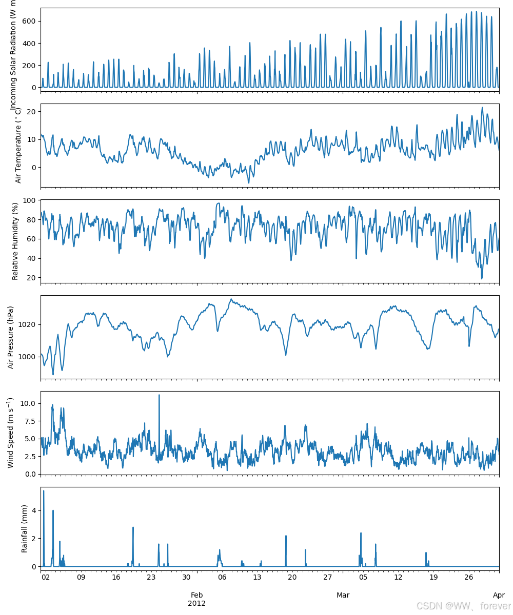

3.1.4. 修改输入参数（Modify Input Parameters）

使用update_config方法修改表面参数。这是参数更改的推荐方法。

# 查看原始表面分数
print("Original surface fractions:")
print(sim.state_init.loc[:, "sfr_surf"])

# 使用update_config修改表面分数
sim.update_config({"initial_states": {"sfr_surf": [0.1, 0.1, 0.2, 0.3, 0.25, 0.05, 0]}})

print("\nModified surface fractions:")
print(sim.state_init.loc[:, "sfr_surf"])

3.1.5. 运行模拟（Run Simulation）

准备好强迫数据和初始条件后，运行SUEWS模拟。run()方法返回一个SUEWSOutput对象，方便访问。

output = sim.run()

print(f"Simulation complete: {len(output.times)} timesteps")
print(f"Output groups: {output.groups}")
print(f"Grids: {output.grids}")

3.1.6. 探索结果：统计（Explore Results: Statistics）

直接通过输出对象的属性访问输出变量。使用pandas的内置方法进行快速的统计摘要。

# 通过SUEWS输出组访问能量平衡变量
df_suews = output.SUEWS

print("Energy balance statistics:")
print(f"  Net radiation (QN): mean = {df_suews['QN'].mean():.1f} W/m2")
print(f"  Sensible heat (QH): mean = {df_suews['QH'].mean():.1f} W/m2")
print(f"  Latent heat (QE): mean = {df_suews['QE'].mean():.1f} W/m2")
print(f"  Storage heat (QS): mean = {df_suews['QS'].mean():.1f} W/m2")

# 详细统计
df_suews.loc[:, ["QN", "QS", "QH", "QE", "QF"]].describe()

输出内容如下：

Energy balance statistics:
  Net radiation (QN): mean = 10.8 W/m2
  Sensible heat (QH): mean = 70.3 W/m2
  Latent heat (QE): mean = 16.1 W/m2
  Storage heat (QS): mean = 16.2 W/m2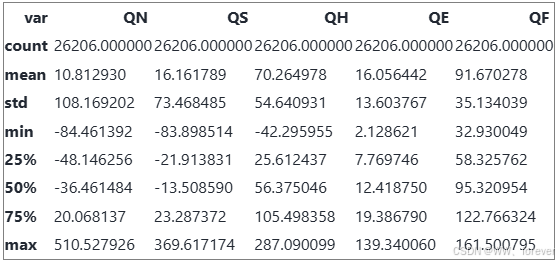

3.1.7. 探索结果：每周能量平衡（Explore Results: Weekly Energy Balance）

绘制一周的表面能量平衡图，以查看昼夜模式。

dict_var_disp = {
    "QN": r"$Q^*$",
    "QS": r"$\Delta Q_S$",
    "QE": "$Q_E$",
    "QH": "$Q_H$",
    "QF": "$Q_F$",
}

# 获取网格ID进行索引
grid = output.grids[0]

# 选择可用数据的第一周进行绘图
start_date = output.times[0]
end_date = start_date + pd.Timedelta(days=7)

fig, ax = plt.subplots(figsize=(10, 4))
(
    df_suews.loc[grid]
    .loc[start_date:end_date, ["QN", "QS", "QE", "QH", "QF"]]
    .rename(columns=dict_var_disp)
    .plot(ax=ax)
)
ax.set_xlabel("Date")
ax.set_ylabel(r"Flux ($\mathrm{W\ m^{-2}}$)")
ax.set_title("Surface Energy Balance (One Week)")
ax.legend()
plt.tight_layout()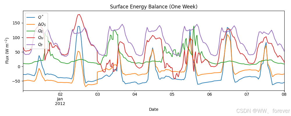

3.1.8. 时间重采样：每日模式（Temporal Resampling: Daily Patterns）

SUEWS以5分钟的间隔运行。重采样为每日值显示季节模式。

rsmp_1d = df_suews.loc[grid].resample("1d")
df_1d_mean = rsmp_1d.mean()
df_1d_sum = rsmp_1d.sum()

# 绘制每日平均能量平衡图
fig, ax = plt.subplots(figsize=(10, 4))
(
    df_1d_mean.loc[:, ["QN", "QS", "QE", "QH", "QF"]]
    .rename(columns=dict_var_disp)
    .plot(ax=ax)
)
ax.set_xlabel("Date")
ax.set_ylabel(r"Mean Flux ($\mathrm{W\ m^{-2}}$)")
ax.set_title("Daily Mean Surface Energy Balance")
ax.legend()
plt.tight_layout()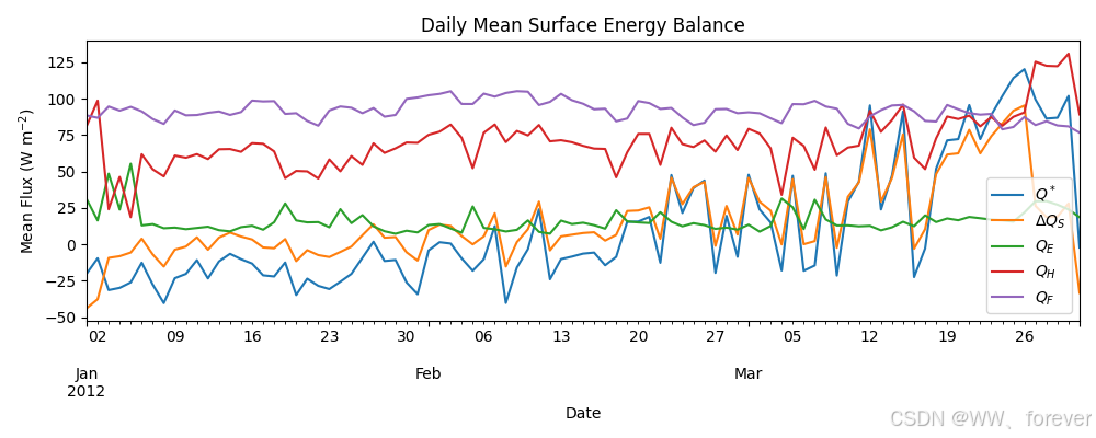

3.1.9. 辐射和水平衡（Radiation and Water Balance）

使用每日聚合值检查辐射组分和水平衡。

dict_var_disp_full = {
    "QN": r"$Q^*$",
    "Kdown": r"$K_{\downarrow}$",
    "Kup": r"$K_{\uparrow}$",
    "Ldown": r"$L_{\downarrow}$",
    "Lup": r"$L_{\uparrow}$",
    "Rain": "$P$",
    "Irr": "$I$",
    "Evap": "$E$",
    "RO": "$R$",
    "TotCh": r"$\Delta S$",
}

fig, axes = plt.subplots(2, 1, figsize=(10, 6), sharex=True)

# 辐射平衡
(
    df_1d_mean.loc[:, ["QN", "Kdown", "Kup", "Ldown", "Lup"]]
    .rename(columns=dict_var_disp_full)
    .plot(ax=axes[0])
)
axes[0].set_ylabel(r"Mean Flux ($\mathrm{W\ m^{-2}}$)")
axes[0].set_title("Radiation Balance")
axes[0].legend()

# 水平衡
(
    df_1d_sum.loc[:, ["Rain", "Irr", "Evap", "RO", "TotCh"]]
    .rename(columns=dict_var_disp_full)
    .plot(ax=axes[1])
)
axes[1].set_xlabel("Date")
axes[1].set_ylabel("Water Amount (mm)")
axes[1].set_title("Surface Water Balance")
axes[1].legend()

plt.tight_layout()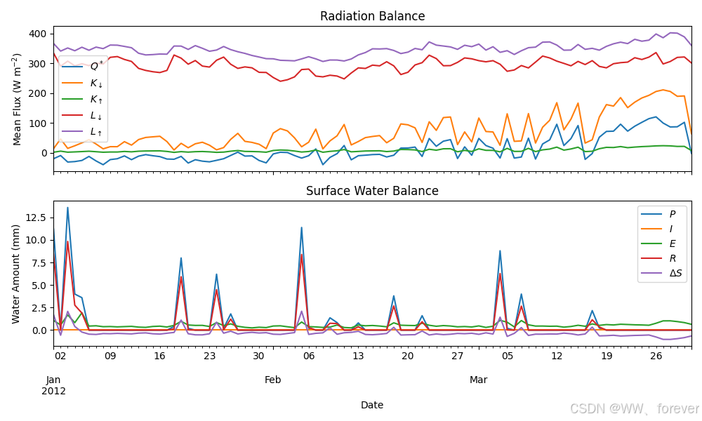

3.1.10. 月度模式（Monthly Patterns）

使用条形图将值聚合到月度，以便进行季节性概述。

df_plot = df_suews.loc[grid].copy()
df_plot.index = df_plot.index.set_names("Month")
rsmp_1M = df_plot.shift(-1).dropna(how="all").resample("1ME")
df_1M_mean = rsmp_1M.mean()
df_1M_sum = rsmp_1M.sum()
# 将索引转换为周期，以获得更好的月份显示
df_1M_mean.index = df_1M_mean.index.to_period("M")
df_1M_sum.index = df_1M_sum.index.to_period("M")

# 月份名字用于标签
name_mon = [x.strftime("%b") for x in rsmp_1M.groups]

fig, axes = plt.subplots(2, 1, sharex=True, figsize=(10, 6))

# 月度能量平衡
(
    df_1M_mean.loc[:, ["QN", "QS", "QE", "QH", "QF"]]
    .rename(columns=dict_var_disp)
    .plot(ax=axes[0], kind="bar")
)
axes[0].set_ylabel(r"Mean Flux ($\mathrm{W\ m^{-2}}$)")
axes[0].set_title("Monthly Surface Energy Balance")
axes[0].legend()

# 月度水平衡
(
    df_1M_sum.loc[:, ["Rain", "Irr", "Evap", "RO", "TotCh"]]
    .rename(columns=dict_var_disp_full)
    .plot(ax=axes[1], kind="bar")
)
axes[1].set_xlabel("Month")
axes[1].set_ylabel("Total Water Amount (mm)")
axes[1].set_title("Monthly Surface Water Balance")
axes[1].xaxis.set_ticklabels(name_mon, rotation=0)
axes[1].legend()

plt.tight_layout()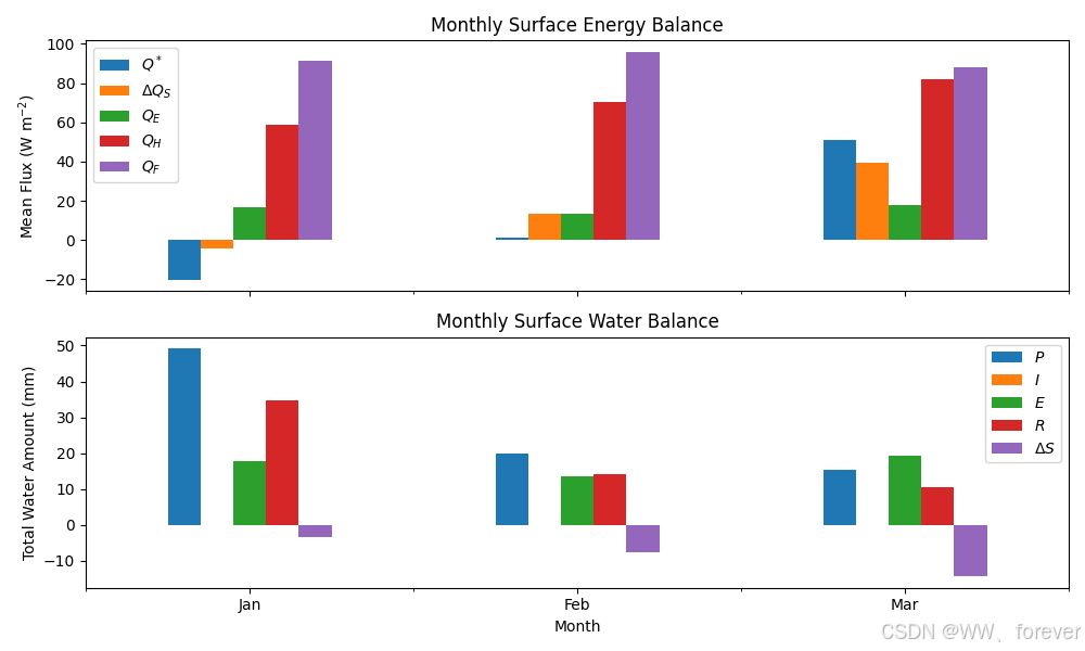

3.1.11. 总结

本教程演示了SUEWS的基本工作流程：

• 使用from_sample_data()加载示例数据
• 使用run()运行模拟，返回SUEWSOutput
• 使用OOP接口探索结果，直观访问变量

涵盖的关键概念包括：

• 能量平衡组成部分：Q*, QH, QE, QS, QF
• 辐射平衡：Kdown, Kup, Ldown, Lup
• 水平衡：Rain, Evap, Runoff, Storage change
• 时间重采样：5分钟至小时，每日，每月

下一步：

• 为您自己的站点设置SUEWS - 为您自己的站点配置SUEWS
• 教程03_impact_studies - 敏感性分析和场景建模

参考

1、官网教程-3.1. SUEWS Quick Start Tutorial