AI 视觉连载7：传统 CV 之高斯滤波实战

本节一起绘制一个可视化的高斯滤波器，同时对一个彩色图像增加高斯噪声，最后通过一个高斯滤波器对图像进行降噪处理。

就像上节说的那样，滤波不是学习重点，下面通过实操了解下原理即可。

可视化高斯滤波器

高斯滤波器符合高斯分布，并且是二维高斯分布，这一点在上一节6、传统 CV 之高斯滤波中已经介绍了。

下面通过 python 来生成一个高斯滤波器，并且对其可视化。

bash 复制代码

import numpy as np
import matplotlib.pyplot as plt
from mpl_toolkits.mplot3d import Axes3D
from scipy.stats import multivariate_normal
# 定义一个高斯滤波器
def gaussian_kernel(size, sigma=1.0):
    kernel = np.fromfunction(
        lambda x, y: (1/ (2 * np.pi * sigma ** 2)) * np.exp(- ((x - size // 2) ** 2 + (y - size // 2) ** 2) / (2 * sigma ** 2)),
        (size, size)
    )
    return kernel / np.sum(kernel)

def plot_gaussian_kernel(kernel):
    fig = plt.figure()

    # 二维图像（像素值）
    ax1 = fig.add_subplot(121)
    ax1.imshow(kernel, cmap='viridis', interpolation='none')
    for i in range(kernel.shape[0]):
        for j in range(kernel.shape[1]):
            ax1.text(j, i, f'{kernel[i, j]:.2f}', ha='center', va='center', color='r')
    ax1.set_title('2D Gaussian Kernel')

    # 三维图像
    ax2 = fig.add_subplot(122, projection='3d')
    x = y = np.arange(0, kernel.shape[0], 1)
    x, y = np.meshgrid(x, y)
    ax2.plot_surface(x, y, kernel, cmap='viridis')
    ax2.set_title('3D Gaussian Kernel')

    plt.show()

def main():
    kernel_size = 5
    sigma = 1.0

    # 生成高斯滤波器
    kernel = gaussian_kernel(kernel_size, sigma)

    # 画出高斯滤波器的二维图像和三维图像
    plot_gaussian_kernel(kernel)

if __name__ == "__main__":
    main()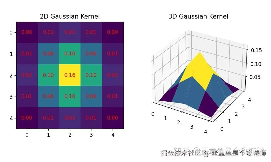

代码结果如上。

左侧为将高斯滤波器中的参数值（权值）采用可视化的二维图像（2D Gaussian Kernel）来展示，每个方块中为滤波器参数。

右侧为将左侧二维图的3D展示，可以看出类似于钟形，类似于高斯正态分布函数围绕着均值部分的旋转。

以上代码和结果在可以在这里获得。

增加高斯模糊

对图像增加高斯模糊，也就是对图像增加一种高斯噪声。

为什么叫高斯噪声呢？是因为噪声数值的分布也符合高斯分布。

高斯噪声是指符合高斯分布（也称正态分布）的随机噪声。在图像处理中，高斯噪声是一种常见的噪声形式。它的分布特点是集中在均值附近，呈现出钟形曲线状的概率密度分布。

可以通过以下程序对一张图像增加高斯噪声（高斯模糊）。

bash 复制代码

import cv2
import numpy as np
import matplotlib.pyplot as plt

def add_gaussian_noise(image, mean=0, sigma=25):
    row, col, ch = image.shape
    gauss = np.random.normal(mean, sigma, (row, col, ch))
    noisy = np.clip(image + gauss, 0, 255)
    return noisy.astype(np.uint8)

def main():
    # 读取原始图像
    original_image = cv2.imread("panda.jpg")

    # 添加高斯噪声
    noisy_image = add_gaussian_noise(original_image)

    # 高斯滤波
    denoised_image = cv2.GaussianBlur(noisy_image, (5, 5), 0)

    # 显示高斯滤波的二维图像
    plt.subplot(131), plt.imshow(cv2.cvtColor(original_image, cv2.COLOR_BGR2RGB)), plt.title('Original Image')
    plt.subplot(132), plt.imshow(cv2.cvtColor(noisy_image, cv2.COLOR_BGR2RGB)), plt.title('Noisy Image')
    plt.subplot(133), plt.imshow(cv2.cvtColor(denoised_image, cv2.COLOR_BGR2RGB)), plt.title('Denoised Image')

    # 保存对比图
    # plt.savefig("gaussian_filter_comparison.png")

    # 显示图像
    plt.show()

if __name__ == "__main__":
    main()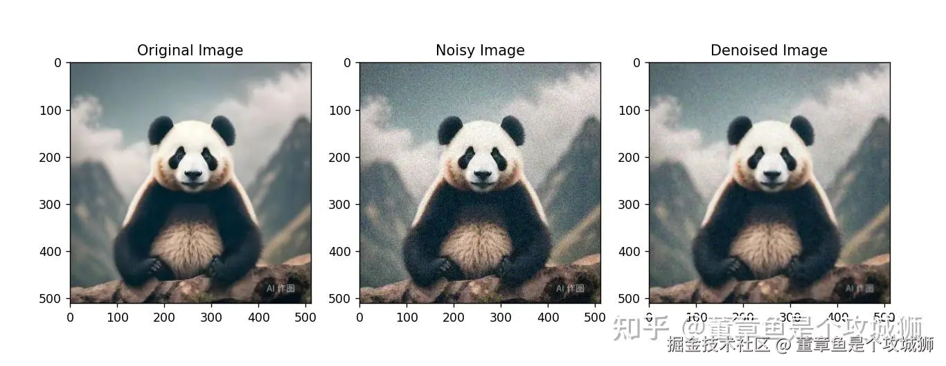

上面三张图，左侧图为原始图像，中间图为增加了高斯噪声之后的图像，可以看到图像中已经出现了噪点。最右侧图像是对中间含噪声的图像进行高斯滤波后的图像。

可以看出滤波之后噪点明显少了一些，并且图像变得稍微平滑，但是和原图相比，清晰度受到了损坏。如果想增加图像的清晰度，可以再通过其他方法（如锐化）来解决。

关于滤波的内容就介绍到这，总的来说，无论是均值滤波还是高斯滤波，都是对图像施加一个正方形的滤波器（带参数的窗口），并将该滤波器窗口中的数值作为权重与图像进行乘累加运算。该滤波器类似于后面要重点学习的卷积核。

本节代码可以在这个链接中获取。