降维是一种常用的数据预处理方法,通过提取关键特征、去除冗余和噪声,在可控的信息损失下提升数据处理效率,并降低时间与计算成本。 正是基于这一需求,主成分分析(Principal components analysis,以下简称PCA) 应运而生,成为数据科学中最经典且应用最广的线性降维方法。
一、PCA思想直观理解
PCA 的核心目标,是在可控的信息损失下,从高维数据中找到一组正交基(即主成分),使其尽可能准确地代表原始数据集。
具体而言,假设我们有 m个样本,每个样本由 n维特征构成。PCA 旨在寻找一个最优投影矩阵,将这些样本从 n维空间映射到 n′维空间(n′<n)。由于降维必然伴随信息丢失,算法的关键在于:如何确保这 n′维的主成分数据,能够最大程度地保留原始数据的变异性(Variance)。
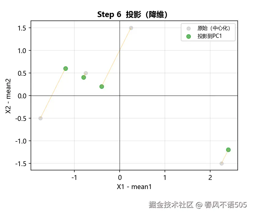
为了更直观地理解这一过程,我们可以观察下方二维数据的降维演示。如下图所示,PCA 首先在 Step 1-2 中对数据进行中心化处理;随后在 Step 3-5 中计算协方差矩阵并寻找方差最大的投影方向(即"最佳视角");最终在 Step 6 中将数据投影至该方向完成降维。
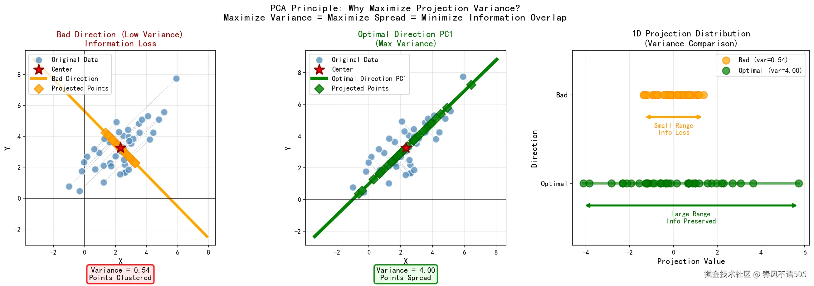
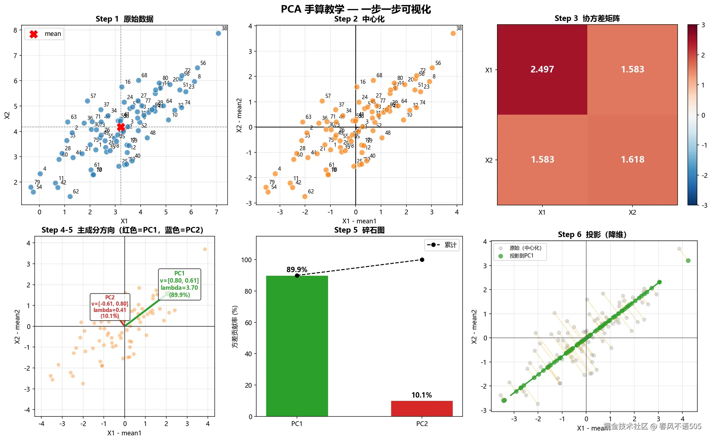 正如上图所示,PCA 的本质就是在空间中寻找一个"最佳视角",使得投影后的数据分布最分散(方差最大), 从而保留最多的原始信息。
值得注意的是,PCA 通常有两种等价的物理解释:一是最大投影方差,二是最小重构误差/最小投影距离。数学上可以证明,这两者最终导向同一个优化目标。接下来,我们将基于最大投影方差理论,对该过程进行严谨的数学推导。此推导将从数据中心化这一基础预处理步骤开始,逐步构建 PCA 的理论框架。
二、PCA的推导:寻找最大投影方差方向
(一) 数据 中心化
设样本矩阵为 X∈Rm×n(m个样本,n维特征),并已预先完成中心化处理(每列均值为 0):
X=x1T x2T ... xmT
数据中心化后,原点即为数据均值。其中,每一个样本向量: xi∈Rn。
(二) 明确 PCA 的优化目标
在此基础上,PCA 的核心任务是寻找一个投影方向 w,使得所有样本在该方向上的投影尽可能分散(即方差最大),从而避免信息重叠。
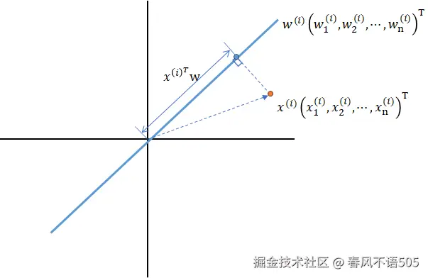
对于任意样本 xi,其在方向 w上的投影坐标为:
zi=xiTw
(三) 推导投影后的方差
基于上述定义,我们构建优化目标。由于原始数据已经中心化,其投影后的均值也为 0:
Ez=0
因此,投影方差可直接表示为样本投影向量的平方和的均值:
Var(z)=Ez2
用样本方差的形式展开:
Var(z)=m−11i=1∑mzi2
将投影公式代入:
Var(z)=m−11i=1∑m(xiTw)2
(四) 矩阵形式展开与协方差矩阵的引入
为了便于利用线性代数工具进行求解,我们需要将上述标量求和形式转化为矩阵形式。注意观察求和项中的平方项:
(xiTw)2
利用矩阵转置的性质,可以进一步改写为二次型的形式:
(xiTw)2=wTxixiTw
将这个结果代回方差公式:
Var(z)=m−11i=1∑mwTxixiTw
由于向量 w 与求和无关,可以将其提取到求和符号外部:
Var(z)=wT(m−11i=1∑mxixiT)w
此时,括号内的部分非常关键------它正是数据的协方差矩阵。
回顾统计学中协方差的定义:
cov(x,y)=m−1∑i=1n(xi−xˉ)(yi−yˉ)
对于多维数据,协方差矩阵 C 是一个对称矩阵,其对角线元素为各维度的方差,非对角线元素为两两维度之间的协方差:
C=cov(x,x)cov(x,y)cov(x,y)cov(y,y)对称阵对角线是方差
其中各元素的计算公式为:
cov(x,y)=m−1∑i=1nxiyicov(x,x)=m−1∑i=1nxi2
将协方差矩阵展开为矩阵乘法的形式:
C= m−1∑i=1nxi2m−1∑i=1nxiyim−1∑i=1nxiyim−1∑i=1nyi2
C=m−11x1y1x2y2x3y3x4y4 x1x2x3x4y1y2y3y4
因此,协方差矩阵可以用数据矩阵简洁地表示为:
C=m−11XXT(X---数据矩阵)
等价写法:
C=m−11∑xixiT
将协方差矩阵 C 代入方差公式,我们得到了一个极其简洁优美的 PCA 的核心表达式------投影方差 Var(z)的矩阵形式:
Var(z)=wTCw
(五) 构建最终的带约束优化模型
显然,为了保留最多信息,PCA 的目标就是最大化这个投影方差。
wmaxwTCw
然而,这个优化问题目前是不严谨的。如果不加任何限制,我们完全可以通过无限增大向量 w 的模长来使得方差无限大,这显然没有实际意义。由于我们只关心投影的"方向",而不关心向量的长度,因此我们需要对 w 施加一个单位长度的约束:
wTw=1
综合以上分析,我们得到了 PCA 最终的带约束优化问题:
wmaxwTCw
s.t.wTw=1
三、模型的求解与物理意义
(一) 引入拉格朗日乘子法
面对带有等式约束的极值问题,最常用的数学工具是拉格朗日乘子法。其核心思想是:通过引入一个新的未知数 λ(称为拉格朗日乘子),将带约束的优化问题转化为无约束的极值问题。构造拉格朗日函数如下:
L(w,λ)=wTCw−λ(wTw−1)
(二) 对方向向量 w 求导
为了找到极值点,我们需要对拉格朗日函数 L(w, λ) 关于向量 w 求梯度,并令其为零。这里需要用到一个矩阵求导的基本公式------对于对称矩阵 A,有:
∂w∂(wTAw)=2Aw
我们将拉格朗日函数拆分为两项:
L(w,λ)=wTCw−λ(wTw−1)
其中:
f1(w)=wTCw
f2(w)=−λ(wTw−1)=−λwTw+λ
对第一项求导:
∂w∂(wTCw)=2Cw
对第二项求导:
∂w∂(−λwTw)=−λ⋅2Iw=−2λw
合并梯度:
∂w∂L=2Cw−2λw
令梯度为零:
2Cw−2λw=0
化简后,我们得到了一个非常经典的等式:
Cw=λw
这正是线性代数中标准的特征值分解方程!也就是说,PCA 的最优投影方向 w 恰好是协方差矩阵 C 的特征向量,而对应的特征值 λ 就是数据在该方向上的投影方差。
(三) 结论与物理意义
上述数学推导将"寻找最大投影方差方向"的几何问题,完美地转化为了"求解协方差矩阵特征值"的代数问题。此转化不仅提供了计算路径,更赋予了各数学符号深刻的物理意义。
让我们回顾整个推导的逻辑链条:
首先,我们确立了优化目标------最大化投影方差:
maxwTCw
然后,通过拉格朗日乘子法,该问题被转化为特征值问题:
Cw=λw
同时,我们还得到了一个重要的等式,它将优化目标值与特征值直接联系起来:
wTCw=λ
在这个结论中,各个数学符号被赋予了深刻的物理意义。协方差矩阵 C 描述了数据的整体分布结构,刻画了原始数据中心化后的"形状"和相关性。特征向量 w 即主成分方向(数据延展的方向),它代表了数据方差最大的投影轴方向。特征值 λ 是对应特征向量的缩放因子,在 PCA 中,它精确地代表了数据投影到该方向上之后的方差大小。
至此,PCA 的理论模型已通过特征值分解得以确立。协方差矩阵的特征向量定义了主成分方向,而特征值则量化了其所承载的方差贡献。在实际应用中,为将此理论转化为可操作的计算步骤,需遵循一套标准化的算法流程。此流程将指导如何从原始数据中提取主成分,实现有效降维。
四、算法流程与实例验证
(一) PCA 完整计算流程
基于上述理论推导,可总结出 PCA 在实际应用中的标准计算步骤。给定数据矩阵 X,其流程如下:
步骤 ①:去均值(中心化)。计算各维度的均值,并将所有数据减去均值:
X−Xˉ
步骤 ②:计算协方差矩阵。使用无偏估计(分母为 m-1),其中 m 为样本数量:
C=m−11XTX
步骤 ③:特征值分解。求解协方差矩阵 C 的特征值和特征向量:
C=QΛQT
步骤 ④:排序与选择。将特征值按从大到小排序,选择前 k 个最大的特征值对应的特征向量。
步骤 ⑤:投影降维。将原始数据投影到选出的 k 个主成分方向上,得到降维后的数据表示。
(二) 手算实例验证
为验证上述流程的有效性,并直观阐明特征值与方差间的量化关系,本文将通过一个包含 4 个二维数据点的实例,进行完整的计算演示。
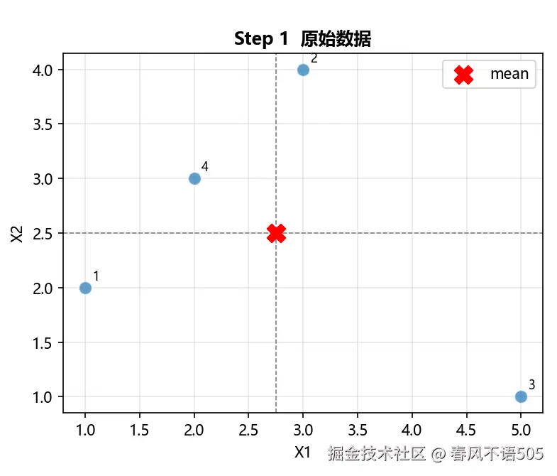
Step 1:数据概览
原始数据包含 4 个二维样本点: (1,2)、(3,4)、(5,1)、(2,3)。数据形状为 (4,2),即 4 个样本、2 个特征维度。
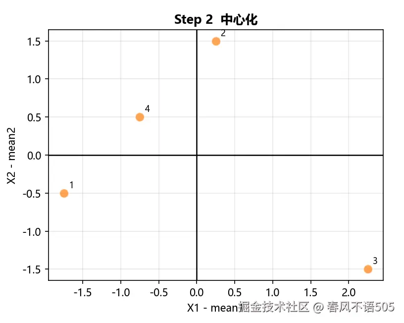
Step 2:数据中心化
均值向量:
μ=(2.75,2.50)
中心化结果(逐点减均值):
(−1.75,−0.50),(0.25,1.50),(2.25,−1.50),(−0.75,0.50)
验证:中心化后各维度均值为 (0,0)。
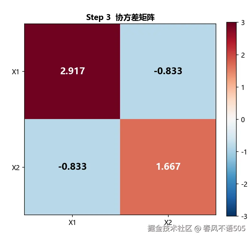
Step 3:计算协方差矩阵
根据公式 Cov=XT⋅X/(n−1),其中 n=4 为样本数,计算得到协方差矩阵:
2.9167−0.8333−0.83331.6667
手动验证: Var(X1)=sum((x1−mean1)2)/(n−1)=8.75/3=2.9167,与矩阵对角线元素一致。
Step 4:特征值分解
求解特征方程 ∣Cov−λI∣=0。利用迹和行列式: trace=2.9167+1.6667=4.5833, det=2.9167×1.6667−(−0.8333)2=4.1667。解二次方程得到:
特征值 λ1=3.3333,对应特征向量 v1=0.8944,−0.4472T
特征值 λ2=1.2500,对应特征向量 v2=0.4472,0.8944T
验证: Cov⋅v1=2.9814,−1.4907, λ1⋅v1=2.9814,−1.4907,两者完全一致。
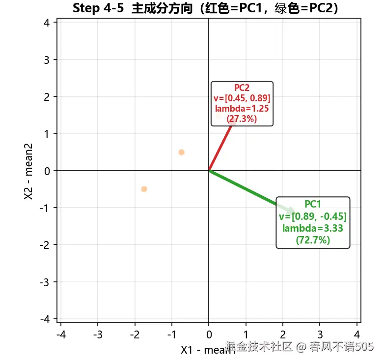
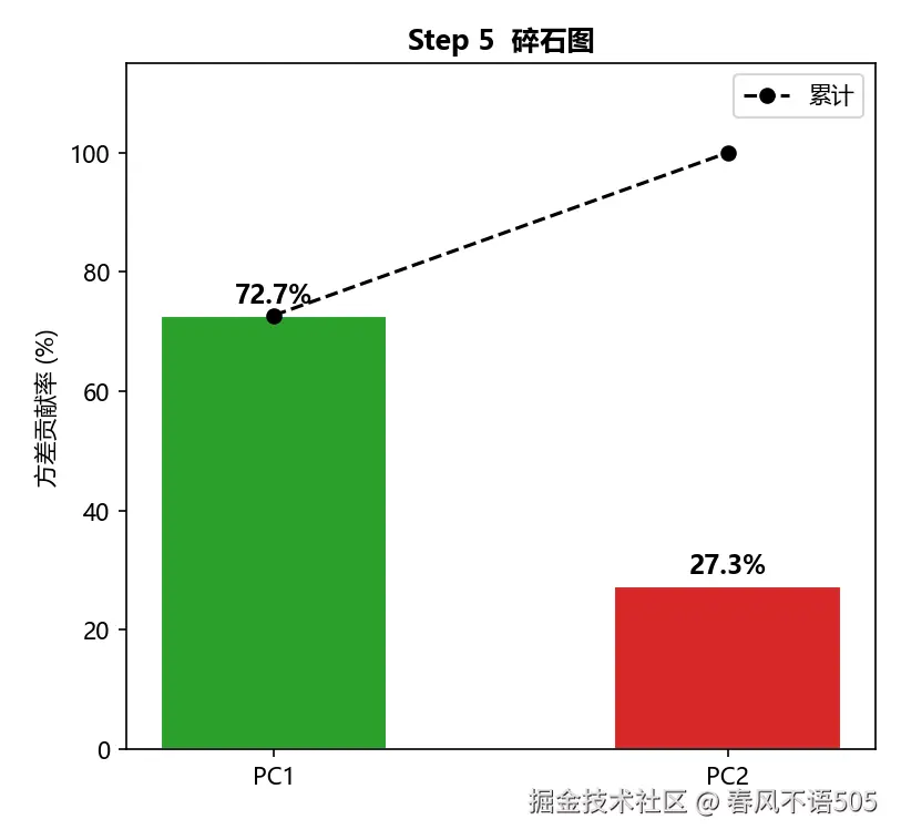
Step 5:按方差贡献率排序
按特征值从大到小排序:PC1 的特征值为 3.3333,方差贡献率为 72.7%;PC2 的特征值为 1.2500,方差贡献率为 27.3%。第一主成分 PC1 捕捉了数据中 72.7% 的信息!
Step 6:投影到主成分空间
将中心化后的数据投影到 PC1 方向向量上。
主成分方向:
v1=0.8944,−0.4472
投影后的一维数据为(点乘):
−1.3416,−0.4472,2.6833,−0.8944
其方差为:
3.3333=λ1
计算这组一维数据的方差,恰好等于 3.3333,与特征值 λ1 完全一致!这完美印证了我们前文推导的核心结论:"特征值代表了数据投影到该方向上的方差大小"。
五、总结
本文系统地阐述了主成分分析(PCA)的核心原理、数学推导及其实践应用。
首先通过几何直观解释了 PCA 作为一种线性降维工具,其本质是在高维空间中寻找最大投影方差的方向,以实现信息损失最小化。
在数学推导层面,展示了如何将原始数据的中心化处理作为起点,通过构建协方差矩阵,利用拉格朗日乘子法将方差最大化问题转化为线性代数中的特征值分解问题。
最后,文章通过标准化的算法五步走流程,结合详尽的手算实例验证,印证了理论推导的正确性。