想要基于OpenGL实现布料模拟,我们需要这几步:
先将布料离散为粒子网格,每个网格单元由两个三角形组成的矩形表示、顶点即粒子,再在粒子间建立水平、垂直、对角及大范围结构弹簧以抵抗拉伸、剪切和大尺度变形;每帧先用上一帧的加速度对粒子做显式欧拉积分更新速度与位置,再对与地面相交的粒子做穿透修正与速度分解(法向反弹、切向摩擦),接着根据三角形面法线累加更新顶点法线用于平滑着色与风力计算,然后清空加速度并按重力、弹簧阻尼力及三角形面上的风力(分配到顶点)重新计算本帧加速度供下一帧使用,最后将顶点位置与法线写入 VBO 完成渲染,从而形成「积分 → 碰撞 → 法线 → 受力」的实时仿真与渲染管线。
接下来我们来逐个学习具体代码实现:
cpp
for (int i = 0; i < height; ++i) {
    for (int j = 0; j < width; ++j) {
        glm::vec3 pos = glm::vec3(-0.1 * width / 2, 0.1 * height / 2, 0) +
            glm::vec3(i) * glm::vec3(0, -0.1, 0) +
            glm::vec3(j) * glm::vec3(0.1, 0, 0);
        Particle* particle = new Particle(pos, glm::vec3(0.1), 0.1);
        particles.push_back(particle);
        positions.push_back(pos);
        if (i == 0) {
            particle->setFix();
            fixedIdx.push_back(i * width + j);
        }
    }
}
我们逐个生成粒子,并用数据结构把各个粒子存储起来,这些粒子的具体坐标都是按照规律生成的,这样就可以构建出粒子网格,第一行 i==0 设为固定点并记录到fixedIdx,相当于布挂在一条边上,只有它们会随布料整体平移/旋转,不参与动力学积分。
cpp
for (int i = 0; i < height - 1; ++i) {
    for (int j = 0; j < width - 1; ++j) {
        int index1 = i * width + j;           // 左上
        int index2 = (i + 1) * width + j;     // 左下
        int index3 = i * width + j + 1;       // 右上
        Particle* p1 = particles[index1], *p2 = particles[index2], *p3 = particles[index3];
        Triangle* triangle = new Triangle(p1, p2, p3);
        indices.push_back(index1); indices.push_back(index2); indices.push_back(index3);
        triangles.push_back(triangle);
    }
}
这里则是我们生成三角形的代码,这里是上三角,可以看到三角形的顶点由我们的粒子组成。
cpp
for (int i = 1; i < height; ++i) {
    for (int j = 0; j < width - 1; ++j) {
        int index1 = i * width + j;           // 左下
        int index2 = i * width + j + 1;       // 右上
        int index3 = (i - 1) * width + j + 1; // 右下
        // ... 同上,new Triangle(p1,p2,p3),push indices 与 triangles
    }
}
下三角,和前者的区别就是index的不同。
每个矩形格由两个三角形覆盖,顶点全部来自粒子,不拷贝位置数据;三角形只持有三个粒子,位置随粒子更新而变。indices存的是粒子下标,用于 EBO 绘制;triangles用于法线累加和风力计算。
cpp
	// 创建水平弹簧阻尼器
	for (int i = 0; i < height; ++i) {
		for (int j = 0; j < width - 1; ++j) {
			int index1 = i * width + j;
			int index2 = i * width + j + 1;
			Particle* p1 = particles[index1];
			Particle* p2 = particles[index2];
			SpringDamper* springDamper = new SpringDamper(p1, p2, 0.1);

			springDampers.push_back(springDamper);
		}
	}

	// 创建垂直弹簧阻尼器
	for (int i = 0; i < height - 1; ++i) {
		for (int j = 0; j < width; ++j) {
			int index1 = i * width + j;
			int index2 = (i + 1) * width + j;
			Particle* p1 = particles[index1];
			Particle* p2 = particles[index2];
			SpringDamper* springDamper = new SpringDamper(p1, p2, 0.1);

			springDampers.push_back(springDamper);
		}
	}

	// 创建对角线(左上到右下)弹簧阻尼器
	for (int i = 0; i < height - 1; ++i) {
		for (int j = 0; j < width - 1; ++j) {
			int index1 = i * width + j;
			int index2 = (i + 1) * width + j + 1;
			Particle* p1 = particles[index1];
			Particle* p2 = particles[index2];
			SpringDamper* springDamper = new SpringDamper(p1, p2, 0.1 * glm::sqrt(2));

			springDampers.push_back(springDamper);
		}
	}

	// 创建对角线(左下到右上)弹簧阻尼器
	for (int i = 1; i < height; ++i) {
		for (int j = 0; j < width - 1; ++j) {
			int index1 = i * width + j;
			int index2 = (i - 1) * width + j + 1;
			Particle* p1 = particles[index1];
			Particle* p2 = particles[index2];
			SpringDamper* springDamper = new SpringDamper(p1, p2, 0.1 * glm::sqrt(2));

			springDampers.push_back(springDamper);
		}
	}

	// 创建大范围水平弹簧阻尼器
	for (int i = 0; i < height - 2; i += 2) {
		for (int j = 0; j < width - 2; j += 2) {
			int index1 = i * width + j;
			int index2 = i * width + j + 2;
			Particle* p1 = particles[index1];
			Particle* p2 = particles[index2];
			SpringDamper* springDamper = new SpringDamper(p1, p2, 0.2);

			springDampers.push_back(springDamper);
		}
	}

	// 创建大范围垂直弹簧阻尼器
	for (int i = 0; i < height - 2; i += 2) {
		for (int j = 0; j < width - 2; j += 2) {
			int index1 = i * width + j;
			int index2 = (i + 2) * width + j;
			Particle* p1 = particles[index1];
			Particle* p2 = particles[index2];
			SpringDamper* springDamper = new SpringDamper(p1, p2, 0.2);

			springDampers.push_back(springDamper);
		}
	}

	// 创建大范围对角线(左上到右下)弹簧阻尼器
	for (int i = 0; i < height - 2; i += 2) {
		for (int j = 0; j < width - 2; j += 2) {
			int index1 = i * width + j;
			int index2 = (i + 2) * width + j + 2;
			Particle* p1 = particles[index1];
			Particle* p2 = particles[index2];
			SpringDamper* springDamper = new SpringDamper(p1, p2, 0.2 * glm::sqrt(2));

			springDampers.push_back(springDamper);
		}
	}

	// 创建大范围对角线(左下到右上)弹簧阻尼器
	for (int i = 2; i < height; i += 2) {
		for (int j = 0; j < width - 2; j += 2) {
			int index1 = i * width + j;
			int index2 = (i - 2) * width + j + 2;
			Particle* p1 = particles[index1];
			Particle* p2 = particles[index2];
			SpringDamper* springDamper = new SpringDamper(p1, p2, 0.2 * glm::sqrt(2));

			springDampers.push_back(springDamper);
		}
	}
每个弹簧会拿两个粒子的序号(具体是哪两个看弹簧类型而定),把对应序号的粒子作为创建弹簧类的参数,丢到弹簧数组中。
cpp
	// 更新法向量和加速度
	updateNormal();
	updateAcceleration();

	// 计算每个粒子的法向量
	for (auto particle : particles) {
		normals.push_back(particle->normal);
	}

	// 生成VAO(顶点数组对象)和VBO(顶点缓冲对象)
	glGenVertexArrays(1, &VAO);
	glGenBuffers(1, &VBO_positions);
	glGenBuffers(1, &VBO_normals);

	// 绑定VAO
	glBindVertexArray(VAO);

	// 绑定VBO - 用于存储顶点位置
	glBindBuffer(GL_ARRAY_BUFFER, VBO_positions);
	glBufferData(GL_ARRAY_BUFFER, sizeof(glm::vec3) * positions.size(), positions.data(), GL_STATIC_DRAW);
	glEnableVertexAttribArray(0);
	glVertexAttribPointer(0, 3, GL_FLOAT, GL_FALSE, 3 * sizeof(GLfloat), 0);

	// 绑定VBO - 用于存储法向量
	glBindBuffer(GL_ARRAY_BUFFER, VBO_normals);
	glBufferData(GL_ARRAY_BUFFER, sizeof(glm::vec3) * normals.size(), normals.data(), GL_STATIC_DRAW);
	glEnableVertexAttribArray(1);
	glVertexAttribPointer(1, 3, GL_FLOAT, GL_FALSE, 3 * sizeof(GLfloat), 0);

	// 生成EBO(元素索引缓冲区),并绑定
	glGenBuffers(1, &EBO);
	glBindBuffer(GL_ELEMENT_ARRAY_BUFFER, EBO);
	glBufferData(GL_ELEMENT_ARRAY_BUFFER, sizeof(unsigned int) * indices.size(), indices.data(), GL_STATIC_DRAW);

	// 解绑VBO
	glBindBuffer(GL_ARRAY_BUFFER, 0);
	glBindVertexArray(0);
先算初始法线和加速度,再把每个粒子的 `position`、`normal` 填入 `positions`、`normals`,创建 VAO、两个 VBO、EBO 并设置顶点属性(location 0 位置,location 1 法线)。这里的初始法线指的是粒子的法线,而粒子的法线的具体来源则是来源于三角形的面法线------我们会基于三角形的边叉积得到面法线,然后我们将这个法线方向直接给到三个顶点作为法线,这样做的理由是为了所谓的平滑着色------提高渲染后的图形的视觉效果。
以上呢就是我们来执行每帧更新之前需要的具体数据了,接下来我们来看怎么进行计算:
cpp
	void Cloth::update() {
		// 更新每个粒子的状态
		for (auto particle : particles) {
			particle->move(0.001);  // 移动粒子
			// ... 后面是碰撞检测
		}
	}
在布料类中执行update,这里的move是执行修改粒子的位置函数,参数则是更新的时间步参数。
cpp
// 移动粒子,更新粒子的速度和位置
void Particle::move(float step) {
    // 如果粒子不是固定的,才进行运动更新
    if (!fixed) {
        // 根据加速度更新速度
        velocity = velocity + step * acceleration;
        // 根据速度更新位置
        position = position + step * velocity;
    }
}
move函数的内容长这样,根据上一帧的加速度更新速度,再根据这一帧更新的速度更新位置。
cpp
//这里转化下坐标,粒子位置在布料局部坐标系,地面在世界坐标系,得转换一下
		glm::vec3 pos = glm::vec3(model * glm::vec4(particle->position, 1));

		// 碰撞检测与反弹处理
		if (land->collide(pos)) {
			//碰撞了,防止下穿透,修正下
			pos[1] = land->top() + 0.01;
			//如果只改速度,不改位置,粒子已经在地面下面,下一帧还会继续穿透,最终还是抖动
			particle->position = glm::vec3(glm::inverse(model) * glm::vec4(pos, 1));

			//速度转换到世界空间,因为碰撞法线在世界空间,所以速度投影必须同空间,w=0是因为速度是方向向量,不受平移影响
			glm::vec3 v = glm::vec3(model * glm::vec4(particle->velocity, 0));
			//垂直于地面的速度(会反弹)
			glm::vec3 vClose = glm::dot(glm::vec3(0, 1, 0), v) * glm::vec3(0, 1, 0);
			//沿地面的速度(会摩擦)
			glm::vec3 vTangent = v - vClose;

			//length(vClose) ≈ 碰撞强度,自定义个0.5f的摩擦系数
			if (vTangent != glm::vec3(0)) {
				//接触越用力,摩擦越大
				float decreaseRatio = glm::min(0.5f * glm::length(vClose), 1.0f);
				vTangent = (1 - decreaseRatio) * vTangent;
			}

			//-0.1f * vClose是在计算反弹恢复系数;1就是完全弹性,0就是完全不弹,可以自己调
			//然后再把速度一转,回到局部空间
			particle->velocity = glm::vec3(glm::inverse(model) * glm::vec4(-0.1f * vClose + vTangent, 0));
		}
......
......

bool Land::collide(glm::vec3 pos) {
	// 计算地面上的一个点(地面位于y=0平面)
	glm::vec3 point = glm::vec3(model * glm::vec4(0, 1, 0, 1));
	// 地面的法向量是(0, 1, 0)
	glm::vec3 normal = glm::vec3(0, 1, 0);

	// 使用点积来检测点是否与地面发生碰撞
	if (glm::dot(pos - point, normal) > 0) {
		// 如果点在地面上方,则没有碰撞
		return false;
	}
	else {
		// 如果点在地面下方,则发生碰撞
		return true;
	}
}

float Land::top() {
	// 返回地面的最高点的y坐标
	return glm::vec3(model * glm::vec4(0, 1, 0, 1))[1];
}
这里是负责检测是否与地面碰撞,如果发生碰撞就进行位置修正和提供反作用力的代码。先把粒子位置和速度用布料的 model 从局部空间变到世界空间,用 land->collide(pos)(点与地面参考点的有符号高度 dot(pos - point, normal) 是否 ≤ 0)判断是否穿透;若穿透则把世界坐标的 y 抬到 land->top() + 0.01 并变回局部写回 particle->position 防止继续下沉,同时在世界空间把速度拆成法向分量和切向分量,法向乘 -0.1 做反弹、切向按与法向速度相关的比例做摩擦衰减,再把合成后的速度用 inverse(model) 变回局部写回 particle->velocity,从而在布料局部坐标系下完成"防穿透 + 反弹 + 摩擦"的碰撞响应。
注意:地面修正的逻辑是:先把粒子变到世界坐标,判断是否穿透;穿透则把位置抬到地面之上,并对"经历位置修正"的粒子做速度响应------法向分量按恢复系数反弹,切向分量按摩擦系数衰减,二者都是直接改速度,而不是施加力。
cpp
//更新法向量为了渲染起来好看,看起来平滑柔软而不是一块一块的
void Cloth::updateNormal() {
	// 更新每个粒子的法向量
	for (auto particle : particles) {
		particle->normal = glm::vec3(0);
	}

	// 更新三角形的法向量
	for (auto triangle : triangles) {
		triangle->updateNormal();
	}

	// 归一化粒子的法向量
	for (auto particle : particles) {
		particle->normal = glm::normalize(particle->normal);
	}
}
这个部分是负责更新粒子法线方向的,正如之前所说,为了实现平滑着色。
cpp
// 更新三角形的法线
void Triangle::updateNormal() {
    // 计算两个边:从 p1 到 p2 和从 p1 到 p3
    glm::vec3 side1 = p2->position - p1->position;
    glm::vec3 side2 = p3->position - p1->position;
    // 通过叉乘计算法线向量,并归一化
    glm::vec3 normal = glm::normalize(glm::cross(side1, side2));

    // 将计算得到的法线添加到每个粒子的法线中
    p1->normal += normal;
    p2->normal += normal;
    p3->normal += normal;
}
上文中调用的更新三角形的法线的函数,逻辑是先更新三角形法线再更新粒子法线。
cpp
void Cloth::updateAcceleration() {
	// 更新每个粒子的加速度
	for (auto particle : particles) {
		particle->clearAcceleration();  // 清除之前的加速度
		particle->applyAcceleration(glm::inverse(model) * glm::vec4(0, -9.8, 0, 0));  // 应用重力加速度
	}

	// 更新弹簧阻尼器的加速度
	for (auto springDamper : springDampers) {
		springDamper->updateAcceleration();
	}

	// 应用风力
	for (auto triangle : triangles) {
		triangle->wind(localWind);
	}
}
然后我们就来更新每个粒子的加速度来,显然我们需要先清零粒子的加速度,不然粒子之前受的力的效果始终不会消失,然后我们优先更新粒子的加速度,然后更新弹簧的加速度,最后应用风力的效果。
cpp
// 更新弹簧阻尼器的加速度
void SpringDamper::updateAcceleration() {
    // 计算当前粒子之间的距离
    float currLength = glm::length(p2->position - p1->position);
    // 计算偏移量:当前长度与静止长度之差
    float deltaX = currLength - restLength;
    glm::vec3 direction;

    // 如果当前长度为 0,设定弹簧方向为 (0, 1, 0),避免除零错误
    if (currLength == 0) {
        direction = glm::vec3(0, 1, 0);
    }
    else {
        // 计算单位向量,表示弹簧的方向
        direction = glm::normalize(p2->position - p1->position);
    }

    // 如果当前长度大于静止长度的 1.2 倍,则进行过度伸展的处理
    if (currLength > 1.2 * restLength) {
        // 计算弹簧中点
        glm::vec3 center = (p2->position + p1->position) / 2.0f;
        // 如果 p1 没有被固定,则将 p1 位置更新为弹簧伸长的适当位置
        if (!p1->fixed) {
            p1->position = center - 0.6f * restLength * direction;
        }
        // 如果 p2 没有被固定,则将 p2 位置更新为弹簧伸长的适当位置
        if (!p2->fixed) {
            p2->position = center + 0.6f * restLength * direction;
        }
    }
    // 如果当前长度小于静止长度的 0.5 倍,则进行过度压缩的处理
    else if (currLength < 0.5 * restLength) {
        // 计算弹簧中点
        glm::vec3 center = (p2->position + p1->position) / 2.0f;
        // 如果 p1 没有被固定,则将 p1 位置更新为弹簧压缩的适当位置
        if (!p1->fixed) {
            p1->position = center - restLength * direction / 4.0f;
        }
        // 如果 p2 没有被固定,则将 p2 位置更新为弹簧压缩的适当位置
        if (!p2->fixed) {
            p2->position = center + restLength * direction / 4.0f;
        }
    }

    // 计算两个粒子之间的相对速度在弹簧方向上的分量
    glm::vec3 vClose = glm::dot(p2->velocity - p1->velocity, direction) * direction;
    // 计算弹簧力和阻尼力
    glm::vec3 force = ks * deltaX * direction + kd * vClose;

    // 将计算得到的力施加到两个粒子上,弹簧力是相反的作用力
    p1->applyForce(force);
    p2->applyForce(-force);
}
先根据两端粒子的位置算出弹簧当前的长度、形变量和方向,若拉得太长或压得太短,就直接在位置层面把两点拉回到"合理距离"附近(硬约束防发散);然后按胡克定律 + 阻尼力算出沿弹簧方向的力,分别以相反方向施加到两个粒子上,通过 applyForce 写入它们的加速度,驱动后续的速度/位置更新。
cpp
// 计算风力对三角形的作用
void Triangle::wind(glm::vec3 vWind) {
// 计算三角形的两个边:从 p1 到 p2 和从 p1 到 p3
glm::vec3 side1 = p2->position - p1->position;
glm::vec3 side2 = p3->position - p1->position;
// 计算三角形的面积,使用叉乘来得到平行四边形的面积,再除以 2 得到三角形面积
float area = glm::length(glm::cross(side1, side2)) / 2.0f;
// 计算三角形的法线
glm::vec3 normal;
if (area == 0) {
normal = glm::vec3(0, 1, 0); // 如果面积为 0(可能是共线的情况),使用默认法线
}
else {
normal = glm::normalize(glm::cross(side1, side2)); // 归一化叉乘结果得到法线
}
// 计算三角形的平均速度
glm::vec3 vTriangle = (p1->velocity + p2->velocity + p3->velocity) / 3.0f;
// 计算相对风速(风速减去三角形的平均速度)
glm::vec3 vClose = vTriangle - vWind;
// 计算与风速方向垂直的面积分量
float crossArea;
if (glm::length(vClose) == 0) {
crossArea = 0; // 如果风速为 0,则没有风力作用
}
else {
// 使用风速与法线的点积来计算垂直于风速的面积分量
crossArea = area * glm::dot(vClose, normal) / glm::length(vClose);
}
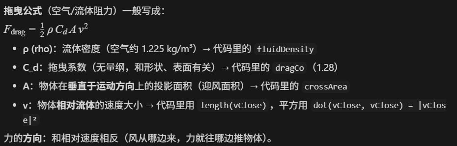
// 计算风力作用于三角形的力,公式为:拖曳力 = -0.5 * 流体密度 * 拖曳系数 * 风速平方 * 面积 * 法线
glm::vec3 force = -fluidDensity * dragCo * glm::dot(vClose, vClose) * crossArea * normal / 2.0f;
// 将风力分配到每个粒子上,假设风力均匀作用于三个粒子
glm::vec3 forceOnParticle = force / 3.0f;
// 对每个粒子施加计算得到的风力
p1->applyForce(forceOnParticle);
p2->applyForce(forceOnParticle);
p3->applyForce(forceOnParticle);
}然后就是执行风力的效果,和之前的情况不同,我们这里需要计算三角形的面积(两条边叉乘结果除以2),先算三角形面积和法线、再算相对风速和迎风面积,用拖曳公式得到三角形所受风力,然后均分到三个顶点上,通过 applyForce 写成粒子加速度,参与下一帧的积分。
这里牵扯到一个拖曳公式:
这样布料模拟中的一个粒子的一帧中执行的内容就完成了打,但我们还差最后的一步。
cpp
// 更新粒子的位置和法向量
	for (int i = 0; i < particles.size(); ++i) {
		positions[i] = particles[i]->position;
	}

	for (int i = 0; i < particles.size(); ++i) {
		normals[i] = particles[i]->normal;
	}

	// 绑定VAO并更新数据
	glBindVertexArray(VAO);

	// 更新顶点位置VBO
	glBindBuffer(GL_ARRAY_BUFFER, VBO_positions);
	glBufferData(GL_ARRAY_BUFFER, sizeof(glm::vec3) * positions.size(), positions.data(), GL_STATIC_DRAW);
	glEnableVertexAttribArray(0);
	glVertexAttribPointer(0, 3, GL_FLOAT, GL_FALSE, 3 * sizeof(GLfloat), 0);

	// 更新法向量VBO
	glBindBuffer(GL_ARRAY_BUFFER, VBO_normals);
	glBufferData(GL_ARRAY_BUFFER, sizeof(glm::vec3) * normals.size(), normals.data(), GL_STATIC_DRAW);
	glEnableVertexAttribArray(1);
	glVertexAttribPointer(1, 3, GL_FLOAT, GL_FALSE, 3 * sizeof(GLfloat), 0);
我们还需要去更新VAO,顶点位置和法线方向的VBO,保证数据的更新,EBO 不变,只更新顶点数据实现动态网格绘制。
如果有人记不住VAO,VBO和EBO这些概念的话:
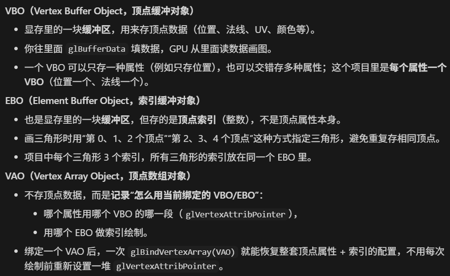
这个项目中两个VBO分别存顶点的位置和法线方向,一个EBO存顶点索引,一个VAO记录如何使用VBO和EBO。
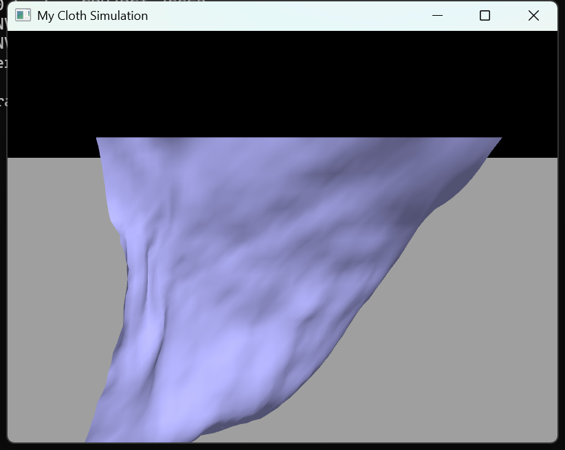
最后展示一下效果: