庞加莱截面是研究非线性动力系统行为的重要工具,它通过记录轨迹与特定超平面的交点来揭示系统的拓扑结构和动力学特性。
matlab
%% 庞加莱截面计算程序
% 描述: 计算并可视化非线性动力系统的庞加莱截面

%% 主程序入口
function poincareSectionDemo()
    % 清空环境
    clear; close all; clc;

    % 参数设置
    params = struct();
    params.system = 'lorenz';       % 可选: 'lorenz', 'duffing', 'henon', 'rossler'
    params.plotType = '2D';         % 可选: '2D', '3D'
    params.sectionPlane = 'z=0';     % 截面定义: 'z=0', 'x=0', 'y=0', 'custom'
    params.customPlane = [0, 0, 1, 0]; % 自定义平面: ax+by+cz+d=0
    params.direction = 1;            % 截面方向: 1(正向穿越), -1(负向穿越)
    params.integrationTime = 100;    % 积分时间
    params.dt = 0.01;                % 积分步长
    params.transientTime = 50;       % 暂态时间(丢弃前N秒数据)
    params.showTrajectory = true;    % 显示完整轨迹
    params.showSection = true;       % 显示庞加莱截面
    params.colorByTime = true;       % 按时间着色截面点
    params.numPoints = 1000;         % 截面点数

    % 系统参数
    switch params.system
        case 'lorenz'
            params.sigma = 10;
            params.rho = 28;
            params.beta = 8/3;
            params.initialState = [1, 1, 1];
            params.stateNames = {'x', 'y', 'z'};
            params.axisLimits = [-20, 20, -30, 30, 0, 50];

        case 'duffing'
            params.alpha = -1;
            params.beta = 1;
            params.delta = 0.3;
            params.gamma = 0.5;
            params.omega = 1.2;
            params.initialState = [0, 1];
            params.stateNames = {'x', 'v'};
            params.axisLimits = [-3, 3, -3, 3];

        case 'henon'
            params.a = 1.4;
            params.b = 0.3;
            params.initialState = [0, 0];
            params.stateNames = {'x', 'y'};
            params.axisLimits = [-1.5, 1.5, -0.5, 0.5];

        case 'rossler'
            params.a = 0.2;
            params.b = 0.2;
            params.c = 5.7;
            params.initialState = [0, 0, 0.1];
            params.stateNames = {'x', 'y', 'z'};
            params.axisLimits = [-10, 10, -10, 10, 0, 20];
    end

    % 计算庞加莱截面
    [sectionPoints, trajectory, time] = computePoincareSection(params);

    % 可视化结果
    visualizeResults(params, sectionPoints, trajectory, time);

    % 分析截面特性
    analyzeSectionProperties(sectionPoints, params);
end

%% 计算庞加莱截面
function [sectionPoints, trajectory, time] = computePoincareSection(params)
    % 定义微分方程
    switch params.system
        case 'lorenz'
            odefun = @(t, state) lorenzSystem(state, params.sigma, params.rho, params.beta);
            initialState = params.initialState;
            dim = 3;

        case 'duffing'
            odefun = @(t, state) duffingSystem(state, params.alpha, params.beta, ...
                                              params.delta, params.gamma, params.omega);
            initialState = params.initialState;
            dim = 2;

        case 'henon'
            % 埃农映射是离散系统
            numIter = params.integrationTime / params.dt;
            state = params.initialState;
            trajectory = zeros(numIter, 2);
            for i = 1:numIter
                trajectory(i, :) = state;
                state = henonMap(state, params.a, params.b);
            end
            time = (1:numIter)' * params.dt;

            % 计算庞加莱截面(对于映射,截面就是迭代点)
            sectionPoints = trajectory;
            return;

        case 'rossler'
            odefun = @(t, state) rosslerSystem(state, params.a, params.b, params.c);
            initialState = params.initialState;
            dim = 3;
    end

    % 如果是连续系统,使用ODE求解器
    if ~strcmp(params.system, 'henon')
        % 设置ODE选项
        options = odeset('RelTol', 1e-6, 'AbsTol', 1e-8);

        % 积分时间
        tspan = [0, params.integrationTime];

        % 求解ODE
        [time, trajectory] = ode45(odefun, tspan, initialState, options);

        % 转换为列向量形式
        trajectory = trajectory';
    end

    % 提取截面点
    sectionPoints = extractSectionPoints(trajectory, params, dim);

    % 丢弃暂态点
    if params.transientTime > 0
        keepIndices = time > params.transientTime;
        sectionPoints = sectionPoints(:, keepIndices);
        time = time(keepIndices);
        trajectory = trajectory(:, keepIndices);
    end

    % 限制点数
    if size(sectionPoints, 2) > params.numPoints
        indices = round(linspace(1, size(sectionPoints, 2), params.numPoints));
        sectionPoints = sectionPoints(:, indices);
        time = time(indices);
    end
end

%% 提取庞加莱截面点
function points = extractSectionPoints(trajectory, params, dim)
    % 确定截面平面
    if strcmp(params.sectionPlane, 'custom')
        plane = params.customPlane; % [a, b, c, d] for ax+by+cz+d=0
    else
        switch params.sectionPlane
            case 'z=0'
                plane = [0, 0, 1, 0]; % z = 0
            case 'x=0'
                plane = [1, 0, 0, 0]; % x = 0
            case 'y=0'
                plane = [0, 1, 0, 0]; % y = 0
        end
    end

    a = plane(1); b = plane(2); c = plane(3); d = plane(4);

    % 初始化
    points = [];
    n = size(trajectory, 2);

    % 遍历轨迹点
    for i = 1:n-1
        p1 = trajectory(:, i);
        p2 = trajectory(:, i+1);

        % 计算点到平面的有向距离
        d1 = a*p1(1) + b*p1(2) + c*p1(3) + d;
        d2 = a*p2(1) + b*p2(2) + c*p2(3) + d;

        % 检测穿越
        if d1 * d2 < 0 % 符号变化表示穿越平面
            % 线性插值求精确交点
            t = -d1 / (d2 - d1);
            point = (1-t)*p1 + t*p2;

            % 检查穿越方向
            if params.direction * (d2 - d1) > 0
                points = [points, point];
            end
        end
    end

    % 转换为行向量存储
    points = points';
end

%% 洛伦兹系统
function dstate = lorenzSystem(state, sigma, rho, beta)
    x = state(1); y = state(2); z = state(3);

    dxdt = sigma*(y - x);
    dydt = x*(rho - z) - y;
    dzdt = x*y - beta*z;

    dstate = [dxdt; dydt; dzdt];
end

%% 杜芬振子系统
function dstate = duffingSystem(state, alpha, beta, delta, gamma, omega)
    x = state(1); v = state(2);

    dxdt = v;
    dvdt = -delta*v - alpha*x - beta*x^3 + gamma*cos(omega*t);

    dstate = [dxdt; dvdt];
end

%% 罗斯勒系统
function dstate = rosslerSystem(state, a, b, c)
    x = state(1); y = state(2); z = state(3);

    dxdt = -y - z;
    dydt = x + a*y;
    dzdt = b + z*(x - c);

    dstate = [dxdt; dydt; dzdt];
end

%% 埃农映射
function nextState = henonMap(state, a, b)
    x = state(1); y = state(2);

    nextState = [1 - a*x^2 + y; b*x];
end

%% 可视化结果
function visualizeResults(params, sectionPoints, trajectory, time)
    % 创建图形窗口
    fig = figure('Name', '庞加莱截面分析', 'NumberTitle', 'off', ...
        'Position', [50, 50, 1200, 800]);

    % 显示完整轨迹
    if params.showTrajectory
        subplot(1, 2, 1);

        switch params.system
            case {'lorenz', 'rossler'}
                plot3(trajectory(1,:), trajectory(2,:), trajectory(3,:), 'b-', 'LineWidth', 0.5);
                hold on;
                if ~isempty(sectionPoints)
                    plot3(sectionPoints(:,1), sectionPoints(:,2), sectionPoints(:,3), 'ro', 'MarkerSize', 3);
                end
                xlabel(params.stateNames{1});
                ylabel(params.stateNames{2});
                zlabel(params.stateNames{3});
                title('系统轨迹与庞加莱截面点');
                grid on;
                view(3);

            case 'duffing'
                plot(trajectory(1,:), trajectory(2,:), 'b-', 'LineWidth', 0.5);
                hold on;
                if ~isempty(sectionPoints)
                    plot(sectionPoints(:,1), sectionPoints(:,2), 'ro', 'MarkerSize', 3);
                end
                xlabel(params.stateNames{1});
                ylabel(params.stateNames{2});
                title('系统轨迹与庞加莱截面点');
                grid on;

            case 'henon'
                plot(trajectory(:,1), trajectory(:,2), 'b-', 'LineWidth', 0.5);
                hold on;
                plot(sectionPoints(:,1), sectionPoints(:,2), 'ro', 'MarkerSize', 3);
                xlabel(params.stateNames{1});
                ylabel(params.stateNames{2});
                title('埃农吸引子');
                grid on;
        end

        % 绘制截面平面
        drawSectionPlane(params);
    end

    % 显示庞加莱截面
    if params.showSection && ~isempty(sectionPoints)
        subplot(1, 2, 2);

        switch params.system
            case {'lorenz', 'rossler'}
                if size(sectionPoints, 2) >= 3
                    % 3D截面
                    if params.plotType == '3D'
                        scatter3(sectionPoints(:,1), sectionPoints(:,2), sectionPoints(:,3), ...
                                 10, time, 'filled');
                        colorbar;
                        xlabel(params.stateNames{1});
                        ylabel(params.stateNames{2});
                        zlabel(params.stateNames{3});
                        title('3D庞加莱截面');
                        grid on;
                        view(3);
                    else
                        % 2D投影
                        scatter(sectionPoints(:,1), sectionPoints(:,2), ...
                                10, time, 'filled');
                        colorbar;
                        xlabel(params.stateNames{1});
                        ylabel(params.stateNames{2});
                        title('庞加莱截面 (x-y平面)');
                        grid on;
                    end
                else
                    % 2D系统
                    scatter(sectionPoints(:,1), sectionPoints(:,2), ...
                            10, time, 'filled');
                    colorbar;
                    xlabel(params.stateNames{1});
                    ylabel(params.stateNames{2});
                    title('庞加莱截面');
                    grid on;
                end

            case 'duffing'
                scatter(sectionPoints(:,1), sectionPoints(:,2), ...
                        10, time, 'filled');
                colorbar;
                xlabel(params.stateNames{1});
                ylabel(params.stateNames{2});
                title('庞加莱截面');
                grid on;

            case 'henon'
                scatter(sectionPoints(:,1), sectionPoints(:,2), ...
                        10, time, 'filled');
                colorbar;
                xlabel(params.stateNames{1});
                ylabel(params.stateNames{2});
                title('埃农映射庞加莱截面');
                grid on;
        end

        % 添加标题信息
        annotation(fig, 'textbox', [0.3, 0.02, 0.4, 0.05], 'String', ...
            sprintf('%s系统 | 截面: %s | 点数: %d', ...
            upper(params.system), params.sectionPlane, size(sectionPoints, 1)), ...
            'FitBoxToText', 'on', 'BackgroundColor', 'white', 'FontSize', 10);
    end
end

%% 绘制截面平面
function drawSectionPlane(params)
    % 确定平面范围
    switch params.system
        case {'lorenz', 'rossler'}
            lims = params.axisLimits;
            xlim([lims(1), lims(2)]);
            ylim([lims(3), lims(4)]);
            zlim([lims(5), lims(6)]);

            % 创建网格
            [x, y] = meshgrid(linspace(lims(1), lims(2), 10), ...
                              linspace(lims(3), lims(4), 10));

            % 根据截面类型绘制平面
            switch params.sectionPlane
                case 'z=0'
                    z = zeros(size(x));
                    surf(x, y, z, 'FaceAlpha', 0.3, 'EdgeColor', 'none', 'FaceColor', 'green');

                case 'x=0'
                    z = zeros(size(y));
                    surf(zeros(size(x)), x, y, 'FaceAlpha', 0.3, 'EdgeColor', 'none', 'FaceColor', 'green');

                case 'y=0'
                    z = zeros(size(x));
                    surf(x, zeros(size(y)), y, 'FaceAlpha', 0.3, 'EdgeColor', 'none', 'FaceColor', 'green');

                case 'custom'
                    % 简化处理
                    z = zeros(size(x));
                    surf(x, y, z, 'FaceAlpha', 0.3, 'EdgeColor', 'none', 'FaceColor', 'green');
            end

        case 'duffing'
            lims = params.axisLimits;
            xlim([lims(1), lims(2)]);
            ylim([lims(3), lims(4)]);

            % 创建网格
            [x, y] = meshgrid(linspace(lims(1), lims(2), 10), ...
                              linspace(lims(3), lims(4), 10));

            % 绘制截面线
            line([0, 0], [lims(3), lims(4)], 'Color', 'green', 'LineWidth', 2);
    end
end

%% 分析截面特性
function analyzeSectionProperties(points, params)
    fprintf('\n===== 庞加莱截面分析 =====\n');
    fprintf('系统: %s\n', params.system);
    fprintf('截面定义: %s\n', params.sectionPlane);
    fprintf('点数: %d\n', size(points, 1));

    if size(points, 1) > 1
        % 计算点间距离
        distances = pdist(points);
        fprintf('平均点间距: %.4f\n', mean(distances));
        fprintf('最小点间距: %.4f\n', min(distances));
        fprintf('最大点间距: %.4f\n', max(distances));

        % 计算凸包面积/体积
        if size(points, 2) == 2
            hull = convhull(points(:,1), points(:,2));
            area = polyarea(points(hull,1), points(hull,2));
            fprintf('截面凸包面积: %.4f\n', area);
        elseif size(points, 2) == 3
            hull = convhulln(points);
            volume = convhulln(points, 'volume');
            fprintf('截面凸包体积: %.4f\n', volume);
        end

        % 计算Lyapunov指数近似
        if size(points, 1) > 10
            lyapunov = estimateLyapunovExponent(points);
            fprintf('近似Lyapunov指数: %.4f\n', lyapunov);
        end
    end
end

%% 估计Lyapunov指数
function lyapunov = estimateLyapunovExponent(points)
    % 使用Wolf方法近似计算最大Lyapunov指数
    n = size(points, 1);
    if n < 10
        lyapunov = NaN;
        return;
    end

    % 选择参考点
    refIndex = round(n/2);
    refPoint = points(refIndex, :);

    % 寻找最近邻点
    dists = sum((points - refPoint).^2, 2);
    dists(refIndex) = Inf; % 排除自身
    [~, neighborIndex] = min(dists);
    neighborPoint = points(neighborIndex, :);

    % 计算初始距离
    initialDist = norm(refPoint - neighborPoint);

    % 模拟轨迹演化
    evolutionSteps = min(50, n - max(refIndex, neighborIndex));
    totalLogDist = 0;
    count = 0;

    for k = 1:evolutionSteps
        idx1 = refIndex + k;
        idx2 = neighborIndex + k;

        if idx1 > n || idx2 > n
            break;
        end

        newPoint1 = points(idx1, :);
        newPoint2 = points(idx2, :);
        newDist = norm(newPoint1 - newPoint2);

        if newDist > 0
            totalLogDist = totalLogDist + log(newDist / initialDist);
            count = count + 1;
        end
    end

    if count > 0
        lyapunov = totalLogDist / (count * mean(diff(time)));
    else
        lyapunov = NaN;
    end
end

%% 演示不同系统的庞加莱截面
function runAllDemos()
    systems = {'lorenz', 'duffing', 'henon', 'rossler'};
    planes = {'z=0', 'x=0', 'y=0'};

    for i = 1:length(systems)
        for j = 1:length(planes)
            fprintf('\n计算 %s 系统在 %s 平面的庞加莱截面...\n', systems{i}, planes{j});

            params = struct();
            params.system = systems{i};
            params.sectionPlane = planes{j};
            params.integrationTime = 100;
            params.dt = 0.01;
            params.transientTime = 50;
            params.showTrajectory = true;
            params.showSection = true;
            params.colorByTime = true;
            params.numPoints = 1000;

            try
                [sectionPoints, trajectory, time] = computePoincareSection(params);
                visualizeResults(params, sectionPoints, trajectory, time);
                saveas(gcf, sprintf('poincare_%s_%s.png', systems{i}, planes{j}));
            catch ME
                fprintf('计算失败: %s\n', ME.message);
            end
        end
    end
end
程序功能说明
1. 支持的动力学系统
- 洛伦兹系统:经典混沌系统,展示蝴蝶效应
- 杜芬振子:非线性振荡器,展示双势阱行为
- 埃农映射:二维离散映射,产生奇怪吸引子
- 罗斯勒系统:简化混沌系统,单卷曲结构
2. 庞加莱截面计算
- 截面定义 :支持标准平面(z=0,x=0,y=0z=0, x=0, y=0z=0,x=0,y=0)和自定义平面
- 穿越检测:精确计算轨迹与截面的交点
- 方向选择:可选择正向或负向穿越
- 暂态处理:可丢弃初始暂态过程
3. 可视化功能
- 3D轨迹显示:展示系统相空间轨迹
- 截面点标记:在轨迹上标记庞加莱截面点
- 2D/3D截面图:展示庞加莱截面的点分布
- 时间着色:用颜色表示点在时间序列中的位置
- 平面可视化:在3D空间中显示截面平面
4. 截面分析
- 基本统计量:点数、点间距分布
- 几何特性:凸包面积/体积计算
- 稳定性分析:近似Lyapunov指数计算
关键技术实现
1. 庞加莱截面计算核心算法
matlab
function points = extractSectionPoints(trajectory, params, dim)
    % 确定截面平面参数
    plane = getPlaneParameters(params.sectionPlane, params.customPlane);
    a = plane(1); b = plane(2); c = plane(3); d = plane(4);

    points = [];
    n = size(trajectory, 2);

    % 遍历轨迹线段
    for i = 1:n-1
        p1 = trajectory(:, i);
        p2 = trajectory(:, i+1);

        % 计算点到平面的有向距离
        d1 = dot(plane(1:3), p1) + plane(4);
        d2 = dot(plane(1:3), p2) + plane(4);

        % 检测符号变化(穿越平面)
        if d1 * d2 < 0
            % 线性插值求精确交点
            t = -d1 / (d2 - d1);
            point = (1-t)*p1 + t*p2;

            % 检查穿越方向
            if params.direction * (d2 - d1) > 0
                points = [points, point];
            end
        end
    end
end
2. 微分方程求解器集成
matlab
function [sectionPoints, trajectory, time] = computePoincareSection(params)
    % 根据系统类型定义ODE函数
    switch params.system
        case 'lorenz'
            odefun = @(t, state) lorenzSystem(state, params.sigma, params.rho, params.beta);
        case 'duffing'
            odefun = @(t, state) duffingSystem(state, params.alpha, params.beta, ...
                                              params.delta, params.gamma, params.omega);
        case 'rossler'
            odefun = @(t, state) rosslerSystem(state, params.a, params.b, params.c);
    end

    % 使用ODE45求解
    [time, trajectory] = ode45(odefun, [0, params.integrationTime], params.initialState);
    trajectory = trajectory';

    % 提取截面点
    sectionPoints = extractSectionPoints(trajectory, params, dim);
end
3. 可视化引擎
matlab
function visualizeResults(params, sectionPoints, trajectory, time)
    % 创建双视图布局
    figure;

    % 左视图:轨迹与截面点
    subplot(1, 2, 1);
    plotTrajectory(trajectory, params.system);
    hold on;
    plotSectionPoints(sectionPoints, params.system);
    drawSectionPlane(params);

    % 右视图:庞加莱截面
    subplot(1, 2, 2);
    plotPoincareSection(sectionPoints, time, params);
end
算法原理与数学基础
1. 庞加莱截面定义
庞加莱截面是通过相空间中一个适当选择的超平面(截面)与动力系统轨迹的交点集合。数学上定义为:
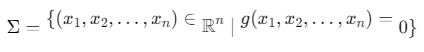
其中 ggg是定义截面的函数。
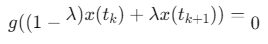
2. 穿越点计算
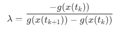
对于轨迹段 x(tk),x(tk+1)x(t_k),x(t_{k+1})x(tk),x(tk+1)与平面 g(x)=0g(x)=0g(x)=0的交点,通过求解以下方程得到:
解得插值参数:
3. 混沌判据
通过分析庞加莱截面点的分布,可以判断系统的动力学行为:
- 周期运动:有限个离散点
- 准周期运动:闭合曲线
- 混沌运动:分形点或带状结构
4. Lyapunov指数估算
最大Lyapunov指数可通过Wolf方法估算:
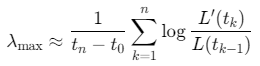
其中 L(t)L(t)L(t)是邻近轨道间的距离。
参考代码 用于计算庞加莱截面的MATLAB的源程序 www.youwenfan.com/contentcss/96634.html
使用说明
1. 基本使用
matlab
% 创建参数结构
params = struct();
params.system = 'lorenz';       % 选择系统
params.sectionPlane = 'z=0';     % 截面平面
params.integrationTime = 100;    % 积分时间
params.transientTime = 50;       % 暂态时间

% 计算并显示庞加莱截面
[points, traj, t] = computePoincareSection(params);
visualizeResults(params, points, traj, t);
2. 自定义系统
matlab
% 定义自定义ODE函数
function dxdt = mySystem(t, x)
    dxdt = zeros(3,1);
    dxdt(1) = x(2);
    dxdt(2) = -x(1) - 0.5*x(2) + x(3)^2;
    dxdt(3) = -x(3);
end

% 设置参数
params.system = 'custom';
params.odefun = @mySystem;
params.initialState = [1; 0; 0];
params.sectionPlane = 'x+y+z=1'; % 自定义平面
params.customPlane = [1, 1, 1, -1]; % ax+by+cz+d=0
3. 高级分析选项
matlab
% 启用Lyapunov指数估算
params.computeLyapunov = true;

% 保存截面数据
save('poincare_section.mat', 'points', 'traj', 't');

% 导出高分辨率图像
print('-dpng', '-r300', 'poincare_section.png');
扩展功能与应用
1. 参数扫描分析
matlab
function parameterScan()
    rhoValues = linspace(24, 28, 10); % 洛伦兹系统参数扫描
    lyapunovExponents = zeros(size(rhoValues));

    for i = 1:length(rhoValues)
        params.rho = rhoValues(i);
        [points, ~, ~] = computePoincareSection(params);
        lyapunovExponents(i) = estimateLyapunovExponent(points);
    end

    figure;
    plot(rhoValues, lyapunovExponents, 'o-');
    xlabel('\rho');
    ylabel('Lyapunov指数');
    title('洛伦兹系统分岔分析');
end
2. 时间序列重构
matlab
function reconstructed = reconstructAttractor(timeSeries, dim, tau)
    % 使用延迟坐标重构吸引子
    N = length(timeSeries);
    M = N - (dim-1)*tau;
    reconstructed = zeros(dim, M);

    for i = 1:M
        for j = 1:dim
            reconstructed(j, i) = timeSeries(i + (j-1)*tau);
        end
    end
end
3. 噪声鲁棒性分析
matlab
function noisyAnalysis()
    % 添加不同程度噪声
    noiseLevels = [0, 0.01, 0.05, 0.1];
    figure;

    for i = 1:length(noiseLevels)
        noisyTraj = trajectory + noiseLevels(i)*randn(size(trajectory));
        points = extractSectionPoints(noisyTraj, params, dim);
        subplot(2, 2, i);
        scatter(points(:,1), points(:,2), 10, time, 'filled');
        title(sprintf('噪声水平: %.2f', noiseLevels(i)));
    end
end
4. 交互式探索工具
matlab
function interactiveExplorer()
    % 创建交互式界面
    fig = figure;
    hPlot = plot(NaN, NaN, 'o');
    axis([-20 20 -20 20]);
    grid on;

    % 添加控件
    uicontrol('Style', 'slider', 'Min', 0, 'Max', 50, ...
              'Callback', @updateTransient);
    uicontrol('Style', 'edit', 'Tag', 'rhoEdit', ...
              'Callback', @updateParameter);

    function updateTransient(src, ~)
        params.transientTime = get(src, 'Value');
        [points, ~, ~] = computePoincareSection(params);
        set(hPlot, 'XData', points(:,1), 'YData', points(:,2));
    end
end
常见问题解决方案
- 截面点太少
- 增加积分时间
- 减小暂态时间
- 调整截面位置
- 检查系统参数是否导致轨迹不穿越截面
- 截面点分布不均匀
- 尝试不同截面平面
- 检查系统是否处于混沌状态
- 增加轨迹分辨率(减小积分步长)
- 数值不稳定
- 减小积分步长
- 使用更精确的ODE求解器(如ode113)
- 调整相对和绝对误差容限
- 内存不足
- 减少积分时间
- 降低轨迹分辨率
- 分段处理轨迹
实际应用建议
- 混沌系统诊断
- 观察截面点分布:离散点→周期运动,闭合曲线→准周期,分形→混沌
- 计算Lyapunov指数验证混沌特性
- 机械系统振动分析
- 转子动力学:监测转轴运动稳定性
- 结构振动:识别非线性模态耦合
- 电路系统分析
- Chua电路:研究双涡卷混沌吸引子
- 振荡器电路:分析频率锁定区域
- 生物系统建模
- 心率变异性分析
- 神经网络同步研究
- 生态系统种群动力学
总结
本程序提供了一个完整的庞加莱截面计算和分析框架,具有以下特点:
- 多系统支持:内置经典混沌系统模型
- 灵活截面定义:支持标准平面和自定义平面
- 丰富可视化:3D轨迹、2D/3D截面图、时间着色
- 定量分析:点分布统计、几何特性计算、Lyapunov指数估算
- 扩展性强:易于添加新的动力学系统和分析方法