使用数据清洗(6种数据填充方式)后的数据集,使用8种算法对某矿石进行分类,类别标签有A、B、C、D这四种标签。
在介绍这8种算法之前,首先要介绍网格搜索,来对算法参数进行调优。
网格搜索
网格搜索也叫超「参数搜索」,比如K-近邻算法的K值需要手动指定参数,这种参数就叫超参数。网格搜索通过预设几组超参数组合,每组超参数都用交叉验证进行评估,从而选出「最优」的参数组合来建立模型。
采用sklearn 模块 GridSearchCV 很好的实现了网格搜索,它可以自动调参,只要把参数输进去,就能给出最优的结果和参数。
python
sklearn.model_selection.GridSearchCV( estimator,param_grid,cv)参数介绍:
estimator:需要使用的分类器
param_grid:需要优化的参数,字典或列表格式{ "n_neighbors": [1, 3, 5] , }
cv:交叉验证次数
返回值属性:
best_params_: (dict)最佳参数
best_score_ : (float)最佳结果
best_estimator_: (estimator)最佳分类器
cv_results_: (dict)交叉验证结果
best_index_: (int)最佳参数的索引
n_splits_:(int)交叉验证的次数
接下来分别在8中算法中使用网格搜索算法来选择最优参数
导入数据集及数据处理
python
import pandas as pd
from sklearn import metrics


train_data = pd.read_excel("../data/训练数据集[中位数].xlsx")
train_data_x = train_data.iloc[:,1:]
train_data_y = train_data.iloc[:,0]

test_data = pd.read_excel('../data/测试数据集[中位数].xlsx')
test_data_x = test_data.iloc[:,1:]
test_data_y = test_data.iloc[:,0]

result_data = {}
逻辑回归算法
python
from sklearn.linear_model import LogisticRegression
from sklearn.model_selection import GridSearchCV

# param_grid = {
#     'penalty':['l1', 'l2','elasticnet','none'],
#     'C':[0.001,0.01,0.1,1,10,100],
#     'solver':['newton-cg','lbfgs','liblinear','sag','saga'],
#     'max_iter':[100,200,500],
#     'multi_class':['auto','ovr','multinomial'],
# }
#
# from sklearn.linear_model import LogisticRegression
#
# logreg = LogisticRegression()
# grid_search = GridSearchCV(logreg,param_grid=param_grid,cv=5)
# grid_search.fit(train_data_x, train_data_y)  # 在训练集上执行网格搜索
# print("Best parameters set found on development set:")  # 输出最佳参数
# print(grid_search.best_params_)

'''  测试结果【训练数据集测试+测试数据集测试】 '''
LR_result = {}
lr = LogisticRegression(C= 0.001,max_iter= 100,penalty=None,solver='lbfgs')
lr.fit(train_data_x,train_data_y)

train_predicted = lr.predict(train_data_x) #训练数据集的预测结果
print('LR的train:\n',metrics.classification_report(train_data_y,train_predicted))
test_predicted = lr.predict(test_data_x)  #测试数据集预测结果
print('LR的test:\n',metrics.classification_report(test_data_y,test_predicted))
a = metrics.classification_report(test_data_y,test_predicted,digits = 6) #digits表示有效位数
b = a.split()

LR_result['recall_0'] = float(b[6])     #添加类别为0的召回率
LR_result['recall_1'] = float(b[11])    #添加类别为1的召回率
LR_result['recall_2'] = float(b[16])    #添加类别为2的召回率
LR_result['recall_3'] = float(b[21])    #添加类别为3的召回率
LR_result['acc'] = float(b[25])     #添加accuracy的结果
result_data = LR_result
print('lr结束')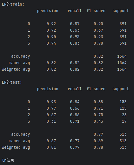
随机森林算法
python
from sklearn.ensemble import RandomForestClassifier
from sklearn.model_selection import GridSearchCV

# param_grid = {
#     'n_estimators': [50, 100, 200],  # 树的数量
#     'max_depth': [None, 10, 20, 30],  # 树的深度
#     'min_samples_split': [2, 5, 10],  # 节点分裂所需的最小样本数
#     'min_samples_leaf': [1, 2, 5],  # 叶子节点所需的最小样本数
#     'max_features': ['auto', 'sqrt', 'log2'],  # 最大特征数
#     'bootstrap': [True, False]  # 是否使用自举样本
# }
#
# # 创建RandomForest分类器实例
# rf = RandomForestClassifier()
# # 创建GridSearchCV对象
# grid_search = GridSearchCV(rf, param_grid, cv=5)
#
# # 在训练集上执行网格搜索
# grid_search.fit(train_data_x, train_data_y)
#
# # 输出最佳参数
# # 输出最佳参数
# print("Best parameters set found on development set:")
# print()
# print(grid_search.best_params_)


''''''
RF_result = {}
rf = RandomForestClassifier(bootstrap=False,
                            max_depth=20,
                            max_features='log2',
                            min_samples_leaf=1,
                            min_samples_split=2,
                            n_estimators=50,
                            random_state=487)

rf.fit(train_data_x, train_data_y)
train_predicted = rf.predict(train_data_x)  # 训练数据集的预测结果
test_predicted = rf.predict(test_data_x)   # 测试数据集的预测结果

print("RF的train:\n", metrics.classification_report(train_data_y, train_predicted))
print("RF的test:\n", metrics.classification_report(test_data_y, test_predicted))
rf_test_report = metrics.classification_report(test_data_y, test_predicted, digits=6)
b = rf_test_report.split()

RF_result['recall_0'] = float(b[6])   # 添加类别为0的召回率
RF_result['recall_1'] = float(b[11])  # 添加类别为1的召回率
RF_result['recall_2'] = float(b[16])  # 添加类别为2的召回率
RF_result['recall_3'] = float(b[21])  # 添加类别为3的召回率
RF_result['acc'] = float(b[25])       # 添加accuracy的结果
result_data['RF'] = RF_result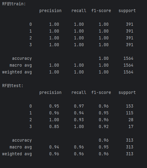
svm算法
python
from sklearn.svm import SVC
from sklearn.model_selection import GridSearchCV

# 定义参数网格
# param_grid = {
#     'C': [0.01, 0.1, 1, 2],  # 惩罚系数
#     'kernel': ['linear', 'poly', 'rbf', 'sigmoid'],  # 核函数类型
#     'degree': [2, 3, 4, 5],  # 多项式核函数的阶数,仅在'poly'核函数下有效
#     'gamma': ['scale', 'auto'] + [1],  # RBF, poly 和 sigmoid 的核函数参数
#     'coef0': [0.1],  # 核函数中的独立项,仅在'poly'和'sigmoid'核函数下有效
# }
#
# svc = SVC()  # 创建SVC分类器实例
#
# # 创建GridSearchCV对象
# grid_search = GridSearchCV(svc, param_grid, cv=5)
#
# # 在训练集上执行网格搜索
# grid_search.fit(train_data_x, train_data_y)
# # 输出最佳参数
# print("Best parameters set found on development set:")
# print()
# print(grid_search.best_params_)

''''''
# 下面的参数均已通过网格搜索算法调优
SVM_result = {}
svm = SVC(C=1, coef0=0.1, degree=4, gamma=1, kernel='poly', probability=True, random_state=100)

svm.fit(train_data_x, train_data_y)
test_predicted = svm.predict(test_data_x)  # 测试数据集的预测结果

print('SVM的test:\n', metrics.classification_report(test_data_y, test_predicted))
a = metrics.classification_report(test_data_y, test_predicted, digits=6)
b = a.split()
print(a)

SVM_result['recall_0'] = float(b[6])   # 添加类别为0的召回率
SVM_result['recall_1'] = float(b[11])  # 添加类别为1的召回率
SVM_result['recall_2'] = float(b[16])  # 添加类别为2的召回率
SVM_result['recall_3'] = float(b[21])  # 添加类别为3的召回率
SVM_result['acc'] = float(b[25])       # 添加accuracy的结果
result_data['SVM'] = SVM_result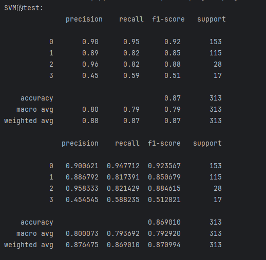
adaboost算法,集成学习,stacking方法
python
from sklearn.ensemble import AdaBoostClassifier
from sklearn.tree import DecisionTreeClassifier
# from sklearn.model_selection import GridSearchCV

# param_grid = {
#     'n_estimators': [50, 100, 200],  # 弱分类器的数量
#     'learning_rate': [0.01, 0.1, 0.5, 1.0],  # 学习率
#     'algorithm': ['SAMME', 'SAMME.R'],  # 提升算法的类型
#     'base_estimator': [DecisionTreeClassifier(max_depth=1), DecisionTreeClassifier(max_depth=2)]
# }

# abf = AdaBoostClassifier(n_estimators=100, random_state=0)  # 创建AdaBoost分类器
# grid_search = GridSearchCV(abf, param_grid, cv=5)  # 创建GridSearchCV对象
# # 在训练集上执行网格搜索
# grid_search.fit(train_data_x, train_data_y)
# # 输出最佳参数
# print("Best parameters set found on development set:\n")
# print(grid_search.best_params_)

''''''
AdaBoost_reslut = {}
abf = AdaBoostClassifier(algorithm='SAMME',
                         estimator=DecisionTreeClassifier(max_depth=2),
                         n_estimators=200,
                         learning_rate=1.0,
                         random_state=0)  # 创建AdaBoost分类器

abf.fit(train_data_x, train_data_y)
train_predicted = abf.predict(train_data_x)  # 训练数据集的预测结果
print('AdaBoost的train:\n', metrics.classification_report(train_data_y, train_predicted))

test_predicted = abf.predict(test_data_x)  # 测试数据集的预测结果
print('AdaBoost的test:\n', metrics.classification_report(test_data_y, test_predicted))

a = metrics.classification_report(test_data_y, test_predicted, digits=6)
b = a.split()

AdaBoost_reslut['recall_0'] = float(b[6])   # 添加类别为0的召回率
AdaBoost_reslut['recall_1'] = float(b[11])  # 添加类别为1的召回率
AdaBoost_reslut['recall_2'] = float(b[16])  # 添加类别为2的召回率
AdaBoost_reslut['recall_3'] = float(b[21])  # 添加类别为3的召回率
AdaBoost_reslut['acc'] = float(b[25])       # 添加accuracy的结果
result_data['AdaBoost'] = AdaBoost_reslut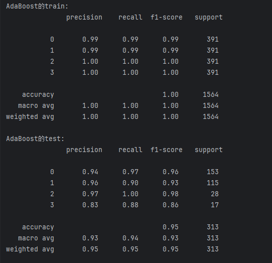
GNB算法实现
python
from sklearn.naive_bayes import GaussianNB

GNB_result = {}

gnb = GaussianNB()  # 创建高斯朴素贝叶斯分类器
gnb.fit(train_data_x, train_data_y)

train_predicted = gnb.predict(train_data_x)  # 训练数据集的预测结果
print('GNB的train:\n', metrics.classification_report(train_data_y, train_predicted))

test_predicted = gnb.predict(test_data_x)  # 测试数据集的预测结果
print('GNB的test:\n', metrics.classification_report(test_data_y, test_predicted))

a = metrics.classification_report(test_data_y, test_predicted, digits=6)
b = a.split()

GNB_result['recall_0'] = float(b[6])  # 添加类别为0的召回率
GNB_result['recall_0'] = float(b[6])   # 添加类别为0的召回率
GNB_result['recall_1'] = float(b[11])  # 添加类别为1的召回率
GNB_result['recall_2'] = float(b[16])  # 添加类别为2的召回率
GNB_result['recall_3'] = float(b[21])  # 添加类别为3的召回率
GNB_result['acc'] = float(b[25])       # 添加accuracy的结果
result_data['GNB'] = GNB_result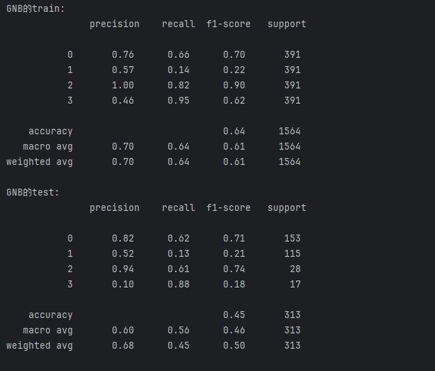
Xgboost算法 集成学习,boosting方法
python
import xgboost as xgb  # 需要额外安装xgboost库
from sklearn.model_selection import GridSearchCV

# # 定义要搜索的参数网格, 此处已经搜索到最优参数, 无需使用此处代码
# param_grid = {
#     'learning_rate': [0.01, 0.05, 0.1],
#     'n_estimators': [50, 100, 200],
#     'max_depth': [3, 5, 7],
#     'min_child_weight': [1, 3, 5],
#     'gamma': [0, 0.1, 0.2],
#     'subsample': [0.6, 0.8, 1.0],
#     'colsample_bytree': [0.6, 0.8, 1.0]
# }
# model = xgb.XGBClassifier(
#     learning_rate=0.1,  # 学习率
#     n_estimators=100,   # 决策树数量
#     max_depth=5,        # 树的最大深度
#     min_child_weight=1, # 叶子节点中最小的样本权重和
#     gamma=0,            # 节点分裂所需的最小损失函数下降值
#     subsample=0.8,      # 训练样本的子样本比例
#     colsample_bytree=1.0 # 每棵树使用特征的子样本比例(根据param_grid补全)
# )
# model = xgb.XGBClassifier(
#     learning_rate=0.1,          # 学习率
#     n_estimators=100,           # 决策树数量
#     max_depth=5,                # 树的最大深度
#     min_child_weight=1,         # 叶子节点中最小的样本权重和
#     gamma=0,                    # 节点分裂所需的最小损失函数下降值
#     subsample=0.8,              # 训练样本的子样本比例
#     colsample_bytree=0.8,       # 每棵树随机采样的列数的占比
#     objective='binary:logistic',# 损失函数类型(对于二分类问题)
#     nthread=4,                  # 使用的线程数(考虑设置为-1来使用所有可用的线程)
#     scale_pos_weight=1,         # 用于处理正负样本不均衡
#     seed=27                     # 随机数种子
# )
# grid_search = GridSearchCV(estimator=model, param_grid=param_grid, cv=3, scoring='accuracy', verbose=1)
# grid_search.fit(train_data_x, train_data_y)

# print("Best parameters found: ", grid_search.best_params_)
# print("Highest accuracy found: ", grid_search.best_score_)


''''''
XGBoost_result = {}
xgb_model = xgb.XGBClassifier(
    learning_rate=0.05,          # 学习率
    n_estimators=200,           # 决策树数量
    num_class=5,                # 类别数量
    max_depth=7,                # 树的最大深度
    min_child_weight=1,         # 叶子节点中最小的样本权重和
    gamma=0,                    # 节点分裂所需的最小损失函数下降值
    subsample=0.6,              # 训练样本的子样本比例
    colsample_bytree=0.8,       # 每棵树随机采样的列数的占比
    objective='multi:softmax',  # 损失函数类型(多分类问题)
    seed=0                      # 随机数种子
)  # 创建XGBoost分类器
xgb_model.fit(train_data_x, train_data_y)

train_predicted = xgb_model.predict(train_data_x)  # 训练数据集的预测结果
print('XGBoost的train:\n', metrics.classification_report(train_data_y, train_predicted))

test_predicted = xgb_model.predict(test_data_x)  # 测试数据集的预测结果
print('XGBoost的test:\n', metrics.classification_report(test_data_y, test_predicted))

a = metrics.classification_report(test_data_y, test_predicted, digits=6)
b = a.split()

XGBoost_result['recall_0'] = float(b[6])   # 添加类别为0的召回率
XGBoost_result['recall_1'] = float(b[11])  # 添加类别为1的召回率
XGBoost_result['recall_2'] = float(b[16])  # 添加类别为2的召回率
XGBoost_result['recall_3'] = float(b[21])  # 添加类别为3的召回率
XGBoost_result['acc'] = float(b[25])       # 添加accuracy的结果
result_data['XGBoost'] = XGBoost_result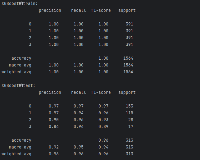
神经网络实现
python
import torch
import torch.nn as nn
import torch.optim as optim
import numpy as np
from sklearn.model_selection import train_test_split

# 定义神经网络结构
class Net(nn.Module):
    def __init__(self):
        super(Net, self).__init__()  # 初始化父类
        self.fc1 = nn.Linear(13, 32)
        self.fc2 = nn.Linear(32, 64)
        self.fc3 = nn.Linear(64, 4)

    def forward(self, x):  # 覆盖父类的方法
        x = torch.relu(self.fc1.forward(x))
        x = torch.relu(self.fc2(x))
        x = self.fc3(x)
        return x

# # 准备数据
# # 转换数据为PyTorch张量
X_train = torch.tensor(train_data_x.values, dtype=torch.float32)
Y_train = torch.tensor(train_data_y.values)
X_test = torch.tensor(test_data_x.values, dtype=torch.float32)
Y_test = torch.tensor(test_data_y.values)
#
# 实例化网络、损失函数和优化器
model = Net()
criterion = nn.CrossEntropyLoss()  # 交叉熵损失函数,适用于多分类任务
optimizer = torch.optim.Adam(model.parameters(), lr=0.001)

def evaluate_model(model, X_data, Y_data, train_or_test):
    size = len(X_data)
    with torch.no_grad():
        predictions = model(X_data)
        correct = (predictions.argmax(1) == Y_data).type(torch.float).sum().item()
        correct /= size
        loss = criterion(predictions, Y_data).item()
        print(f"{train_or_test}: \t Accuracy: {100 * correct}%")
    return correct

epochs = 15000
accs = []
for epoch in range(epochs):  # 训练网络
    optimizer.zero_grad()  # 梯度的初始化
    outputs = model(X_train)

    loss = criterion(outputs, Y_train)
    loss.backward()
    optimizer.step()

    if (epoch + 1) % 100 == 0:
        print(f'Epoch [{epoch + 1}/{epochs}], Loss: {loss.item():.4f}')
        train_acc = evaluate_model(model, X_train, Y_train, 'train')
        test_acc = evaluate_model(model, X_test, Y_test, 'test')
        accs.append(test_acc*100)

net_result = {}
net_result['acc'] = max(accs)
result_data['net'] = net_result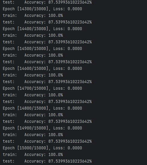
CNN卷积神经网络
python
import torch
import torch.nn as nn
import torch.optim as optim
import numpy as np


# 定义一维卷积神经网络模型
class ConvNet(nn.Module):
    def __init__(self, num_features, hidden_size, num_classes):
        super(ConvNet, self).__init__()
        self.conv1 = nn.Conv1d(in_channels=1, out_channels=16, kernel_size=3, padding=1)
        self.conv2 = nn.Conv1d(in_channels=16, out_channels=32, kernel_size=3, padding=1)
        self.conv3 = nn.Conv1d(in_channels=32, out_channels=64, kernel_size=3, padding=1)
        self.relu = nn.ReLU()
        self.fc = nn.Linear(64, num_classes)

    def forward(self, x):#x[1472*1*13]
        # 由于Conv1d期望的输入维度是(batch_size, channels, length),我们需要增加一个维度
        x = x.unsqueeze(1)  # 增加channels维度
        x = self.conv1(x)
        x = self.relu(x)
        x = self.conv2(x)
        x = self.relu(x)
        x = self.conv3(x)
        x = self.relu(x)
        x = x.mean(dim=2)  # 这里使用平均池化作为简化操作
        x = self.fc(x)
        return x

hidden_size = 10
num_classes = 4
model = ConvNet(13, hidden_size, num_classes)
criterion = nn.CrossEntropyLoss()
optimizer = optim.Adam(model.parameters(), lr=0.001)

# 训练模型
num_epochs = 15000
accs = []
for epoch in range(num_epochs):
    outputs = model(X_train)    # 前向传播
    loss = criterion(outputs, Y_train)
    optimizer.zero_grad()       # 反向传播和优化
    loss.backward()
    optimizer.step()

    if (epoch + 1) % 100 == 0:  #每隔100次打印训练结果
        print(f'Epoch [{epoch + 1}/{num_epochs}], Loss: {loss.item():.4f}')

        # 测试模型
        with torch.no_grad():
            predictions = model(X_train)
            predicted_classes = predictions.argmax(dim=1)
            accuracy = (predicted_classes == Y_train).float().mean()
            print(f'Train Accuracy: {accuracy.item() * 100:.2f}%')

            predictions = model(X_test)
            predicted_classes = predictions.argmax(dim=1)
            accuracy = (predicted_classes == Y_test).float().mean()
            print(f'Test Accuracy: {accuracy.item() * 100:.2f}%')
            accs.append(accuracy*100)
cnn_result = {}
cnn_result['acc'] = max(accs).item()
result_data['cnn'] = cnn_result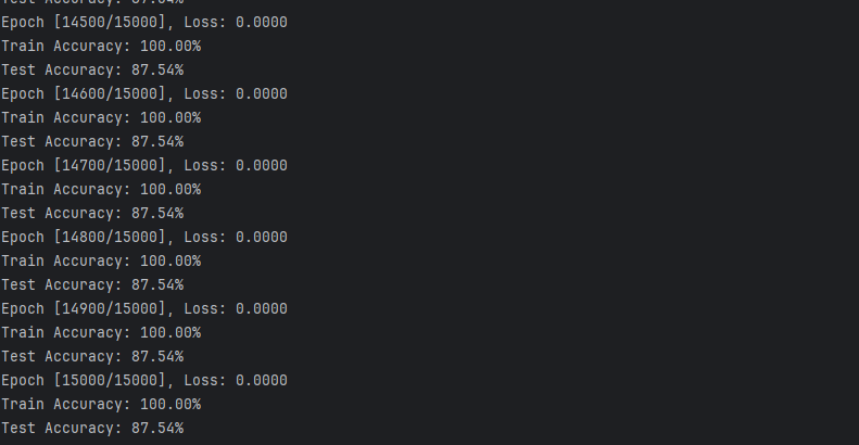
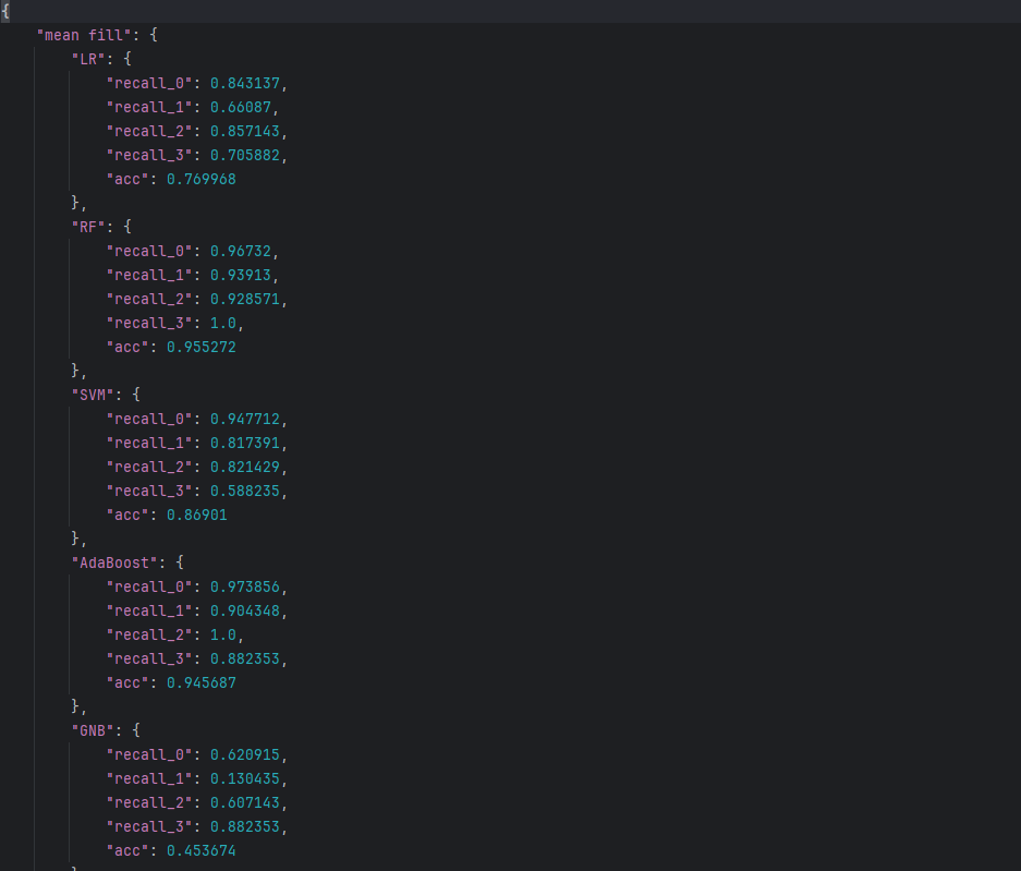
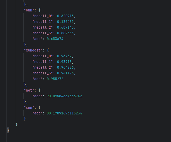
总结
记录以上8种算法各类别标签召回率及准确度
python
import json#数据格式,网络传输。保存提取json类型的数据。  csv:表格类型的数据
# 使用 'w' 模式打开文件,确保如果文件已存在则会被覆盖,
result = {}
result['mean fill'] = result_data
with open(r'../data/平均值填充result.json', 'w', encoding='utf-8') as file:
    # 使用 json.dump() 方法将字典转换为 JSON 格式并写入文件,JSON一般来是字典
    json.dump(result, file, ensure_ascii=False, indent=4)