注:本文为 "浮点数运算" 相关译文,机翻未校。
略作重排,如有内容异常,请看原文。
csdn 篇幅所限,分篇连载。
4. Errol1: Fast & More Optimal
4. Errol1:快速且更优
Our first contribution is the Errol1 conversion algorithm, which instantiates the generic convert (Figure 2) with a novel H P HP HP implementation that simultaneously improves the accuracy and performance of conversion. The performance benefits come from implementing H P HP HP numbers using Knuth's double-double representation 9 and by developing novel algorithms for efficiently performing the key operations over double-doubles that are needed for conversion. Surprisingly, the double-double representation also improves the accuracy of conversion as it lets Errol1 compute the narrow and wide intervals more accurately, thereby shrinking the uncovered intervals and increasing the likelihood that the shortest number in the narrow interval is indeed the optimal result.
本文第一项贡献是 Errol1 转换算法,它用全新的 H P HP HP 实现实例化通用 convert 算法(图 2),同时提升转换精度与性能。性能提升源于:用高德纳双-双精度表示 9 实现 H P HP HP 数值,并设计全新算法高效执行转换所需的双-双精度核心运算。出乎意料的是,双-双精度表示还提升了转换精度,使 Errol1 更精确地计算窄、宽区间,缩小未覆盖区间,提升窄区间内最短数即为最优结果的概率。
Next, we describe double-double based H P HP HP values (§ 4.1) and how Errol1 uses them to implement the key narrow_interval (§ 4.2) and digits (§ 4.3) procedures of Figure 2. These procedures require fast and accurate implementations of specific arithmetic operations over H P HP HP numbers (§ 4.4), and finally we show how we ensure accuracy in the presence of rounding error (§ 4.5). For the remainder of the paper, the H P HP HP type refers to double-double floating-point numbers.
下文介绍基于双-双精度的 H P HP HP 数值(§ 4.1),以及 Errol1 如何用其实现图 2 中的核心过程 narrow_interval(§ 4.2)与 digits(§ 4.3)。这些过程需要快速且精确地实现 H P HP HP 数值上的特定算术运算(§ 4.4),最后说明如何在舍入误差存在时保证精度(§ 4.5)。本文后续部分中, H P HP HP 类型均指双-双精度浮点数。
4.1 Double-Double Representation
4.1 双-双精度表示
We represent double-double numbers (of type H P HP HP) as a pair of native floating-point values (of type F P FP FP). That is,
双-双精度数(类型 H P HP HP)用一对原生浮点数值(类型 F P FP FP)表示,即:
type H P = ( F P , F P ) 类型 H P = ( F P , F P ) \text{type } HP = (FP, FP)\\ \text{类型 } HP = (FP, FP) type HP=(FP,FP)类型 HP=(FP,FP)
H P HP HP values are written as < v ^ b , v ^ δ > <\hat{v}b, \hat{v}\delta> <v^b,v^δ> where the first element v ^ b \hat{v}b v^b is a base value corresponding to the nearest approximation of the target H P HP HP value, and the second element v ^ δ \hat{v}\delta v^δ is an offset value corresponding to the difference between the target value and the base. Thus, the H P HP HP value v ˉ \bar{v} vˉ represented by < v ^ b , v ^ δ > <\hat{v}b, \hat{v}\delta> <v^b,v^δ> is the sum:
H P HP HP 数值记为 < v ^ b , v ^ δ > <\hat{v}b, \hat{v}\delta> <v^b,v^δ>,其中第一个元素 v ^ b \hat{v}b v^b 是基值 ,为目标 H P HP HP 值的最近近似;第二个元素 v ^ δ \hat{v}\delta v^δ 是偏移值 ,为目标值与基值的差。因此, < v ^ b , v ^ δ > <\hat{v}b, \hat{v}\delta> <v^b,v^δ> 表示的 H P HP HP 值 v ˉ \bar{v} vˉ 为和:
v ˉ ≐ v ^ b + v ^ δ \bar{v} \doteq \hat{v}b + \hat{v}\delta vˉ≐v^b+v^δ
Our pair-based representation doubles the precision of the native representation (e.g. if the native F P FP FP has 53 bits of precision, then our H P HP HP has 106 bits of precision). Figure 5 shows how the real 0.2 is represented as a native 8-bit F P FP FP and as a 16-bit H P HP HP value; the latter approximates the real more faithfully.
这种成对表示将原生精度翻倍(例如原生 F P FP FP 为 53 位精度,则 H P HP HP 为 106 位精度)。图 5 展示实数 0.2 分别用原生 8 位 F P FP FP 与 16 位 H P HP HP 表示的结果,后者对实数的近似更精确。
Non-Overlapping Invariant. Let v ^ b \hat{v}b v^b and v ^ δ \hat{v}\delta v^δ be two p p p-bit F P FP FP values. We say that < v ^ b , v ^ δ > <\hat{v}b, \hat{v}\delta> <v^b,v^δ> is non-overlapping if e b ≥ e δ + p e_b \ge e_\delta + p eb≥eδ+p where e b e_b eb and e δ e_\delta eδ are the exponents of v ^ b \hat{v}b v^b and v ^ δ \hat{v}\delta v^δ, respectively. This implies the weaker statement ∣ v ^ b ∣ > ∣ v ^ δ ∣ 2 p − 1 |\hat{v}b| > |\hat{v}\delta| 2^{p-1} ∣v^b∣>∣v^δ∣2p−1 that relates the magnitudes of v ^ b \hat{v}b v^b and v ^ δ \hat{v}\delta v^δ. Our algorithms maintain the invariant that in any H P HP HP value < v ^ b , v ^ δ > <\hat{v}b, \hat{v}\delta> <v^b,v^δ>, the components v ^ b \hat{v}b v^b and v ^ δ \hat{v}\delta v^δ are non-overlapping to ensure the most faithful representation of the target real number.
非重叠不变式 :设 v ^ b \hat{v}b v^b 与 v ^ δ \hat{v}\delta v^δ 为两个 p p p 位 F P FP FP 值。若 e b ≥ e δ + p e_b \ge e_\delta + p eb≥eδ+p( e b e_b eb、 e δ e_\delta eδ 分别为 v ^ b \hat{v}b v^b、 v ^ δ \hat{v}\delta v^δ 的指数),则称 < v ^ b , v ^ δ > <\hat{v}b, \hat{v}\delta> <v^b,v^δ> 非重叠。该条件蕴含更弱的量级关系 ∣ v ^ b ∣ > ∣ v ^ δ ∣ 2 p − 1 |\hat{v}b| > |\hat{v}\delta| 2^{p-1} ∣v^b∣>∣v^δ∣2p−1。本文算法始终保持不变式:任意 H P HP HP 值 < v ^ b , v ^ δ > <\hat{v}b, \hat{v}\delta> <v^b,v^δ> 的分量 v ^ b \hat{v}b v^b 与 v ^ δ \hat{v}\delta v^δ 非重叠,以保证对目标实数的最精确表示。
4.2 Step 1: Compute Narrow Interval
4.2 步骤 1:计算窄区间
The narrow interval computation, summarized in Figure 6, is split into three distinct phases: exponent estimation, boundary computation, and exponent rectification. Each phase uses various H P HP HP arithmetic operations. We defer the implementation of these operations and the errors they incur to § 4.4.
窄区间计算总结于图 6,分为三个独立阶段:指数估计、边界计算、指数修正。每个阶段使用多种 H P HP HP 算术运算。这些运算的实现与误差分析放在 § 4.4。
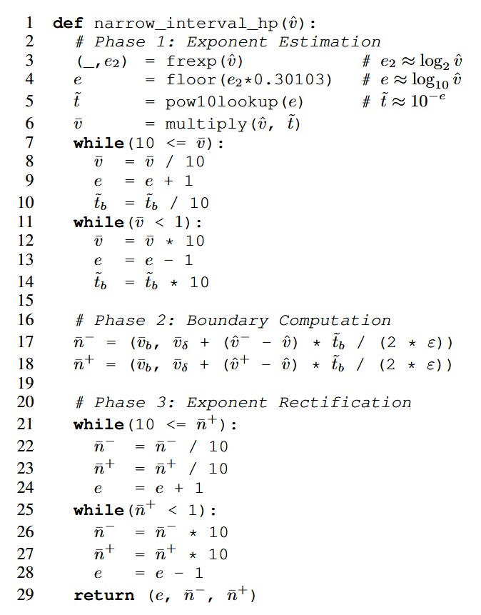
Figure 6: Errol1: Computing the Scaled Narrow Interval.
图 6:Errol1:计算缩放窄区间
Phase 1: Exponent Estimation. Unlike the description in Figure 2, Errol1 first estimates the exponent directly from the input v ^ \hat{v} v^ before computing the boundaries. The estimate optimizes performance by allowing Errol1 to use a fast lookup table to avoid several slow multiplications (by 10). However, as the estimated exponent may be incorrect, it is later rectified in the third phase.
阶段 1:指数估计 :与图 2 描述不同,Errol1 在计算边界前先直接从输入 v ^ \hat{v} v^ 估计指数。该估计通过快速查表避免多次缓慢的乘 10 运算,优化性能。但估计的指数可能不准确,因此在第三阶段修正。
The initial exponent estimation is shown on lines 2--14. The exponent is directly estimated from the input v ^ \hat{v} v^: the frexp function returns the binary exponent and is scaled by log 10 2 ≈ 0.30103 \log_{10} 2 \approx 0.30103 log102≈0.30103 to provide a rough estimation of log 10 v ^ \log_{10} \hat{v} log10v^. The value of 10 − e 10^{-e} 10−e is stored as an H P HP HP value in a lookup table and retrieved on line 5. The values v ^ \hat{v} v^ (an F P FP FP) and 10 − e 10^{-e} 10−e (an H P HP HP) are multiplied to produce a scaled input v ˉ \bar{v} vˉ (an H P HP HP) on line 6. At the end of line 6, the value has been scaled by 10 − e 10^{-e} 10−e (as stored in t ˉ \bar{t} tˉ).
初始指数估计见第 2--14 行。指数直接从输入 v ^ \hat{v} v^ 估计:frexp 函数返回二进制指数,乘以 log 10 2 ≈ 0.30103 \log_{10} 2 \approx 0.30103 log102≈0.30103 得到 log 10 v ^ \log_{10} \hat{v} log10v^ 的粗略估计。 10 − e 10^{-e} 10−e 以 H P HP HP 数值形式存于查表,第 5 行取出。第 6 行将 v ^ \hat{v} v^( F P FP FP 类型)与 10 − e 10^{-e} 10−e( H P HP HP 类型)相乘,得到缩放输入 v ˉ \bar{v} vˉ( H P HP HP 类型)。第 6 行结束时,数值已按 10 − e 10^{-e} 10−e(存于 t ˉ \bar{t} tˉ)缩放。
The lookup table for 10 − e 10^{-e} 10−e can only contain values in the range 10 − 291 , 10 308 10\^{-291}, 10\^{308} 10−291,10308 in order to prevent overflow or underflow of an H P HP HP value. Consequently, input values below 10 − 308 10^{-308} 10−308 or above 10 291 10^{291} 10291 are not successfully scaled into the range [1, 10). Instead, the two loops on lines 6--13 check and incrementally multiply or divide by ten in order to completely scale v ˉ \bar{v} vˉ, by adjusting the exponent e e e and the base component of t ˉ \bar{t} tˉ; the offset is not used later.
为避免 H P HP HP 数值溢出或下溢, 10 − e 10^{-e} 10−e 查表仅包含 10 − 291 , 10 308 10\^{-291}, 10\^{308} 10−291,10308 范围内的值。因此,小于 10 − 308 10^{-308} 10−308 或大于 10 291 10^{291} 10291 的输入无法直接缩放到 [1, 10) 区间。第 6--13 行的两个循环检查并逐次乘/除 10,完整缩放 v ˉ \bar{v} vˉ,同时调整指数 e e e 与 t ˉ \bar{t} tˉ 的基值分量;偏移值后续不再使用。
Phase 2: Boundary Computation. The boundaries n ˉ − \bar{n}^- nˉ− and n ˉ + \bar{n}^+ nˉ+ are computed from the original input v ^ \hat{v} v^ and scaled input v ˉ \bar{v} vˉ on lines 17 and 18. Using the definition of the scaled upper boundary n ˉ + \bar{n}^+ nˉ+, its computation directly follows from the calculation
阶段 2:边界计算 :第 17--18 行从原始输入 v ^ \hat{v} v^ 与缩放输入 v ˉ \bar{v} vˉ 计算边界 n ˉ − \bar{n}^- nˉ− 与 n ˉ + \bar{n}^+ nˉ+。根据缩放上边界 n ˉ + \bar{n}^+ nˉ+ 的定义,其计算直接推导如下:
n ˉ + ≐ v ˉ + v ˉ + 2 = v ^ + v ^ + 2 × 10 − e = 2 v ^ + v ^ + − v ^ 2 × 10 − e = v ^ × 10 − e + v ^ + − v ^ 2 × 10 − e = v ˉ + v ^ + − v ^ 2 × t ^ b \begin{aligned} \bar{n}^+ &\doteq \frac{\bar{v}+\bar{v}^+}{2} \\ &= \frac{\hat{v}+\hat{v}^+}{2} \times 10^{-e} \\ &= \frac{2 \hat{v}+\hat{v}^+-\hat{v}}{2} \times 10^{-e} \\ &= \hat{v} \times 10^{-e}+\frac{\hat{v}^+-\hat{v}}{2} \times 10^{-e} \\ &= \bar{v}+\frac{\hat{v}^+-\hat{v}}{2} \times \hat{t}_b \end{aligned} nˉ+≐2vˉ+vˉ+=2v^+v^+×10−e=22v^+v^+−v^×10−e=v^×10−e+2v^+−v^×10−e=vˉ+2v^+−v^×t^b
where the last equality arises as v ˉ \bar{v} vˉ and t ^ b \hat{t}b t^b are equal to v ^ × 10 − e \hat{v} \times 10^{-e} v^×10−e and 10 − e 10^{-e} 10−e, respectively. Typically, summing the first term ( v ˉ \bar{v} vˉ) and the second term would require a full addition between two H P HP HP numbers. However, the second term is extremely small compared to the first due to the small difference between v ^ \hat{v} v^ and v ^ + \hat{v}^+ v^+ and so the second term can be directly added to the offset component v ^ δ \hat{v}\delta v^δ. The same process applies to computing the lower boundary n ˉ − \bar{n}^- nˉ− by substituting the successor v ^ + \hat{v}^+ v^+ with the predecessor v ^ − \hat{v}^- v^−.
最后一个等号成立是因为 v ˉ = v ^ × 10 − e \bar{v} = \hat{v} \times 10^{-e} vˉ=v^×10−e, t ^ b = 10 − e \hat{t}b = 10^{-e} t^b=10−e。通常,第一项 v ˉ \bar{v} vˉ 与第二项相加需要两个 H P HP HP 数的完整加法。但由于 v ^ \hat{v} v^ 与 v ^ + \hat{v}^+ v^+ 差值极小,第二项远小于第一项,因此可直接加到偏移分量 v ^ δ \hat{v}\delta v^δ 上。计算下边界 n ˉ − \bar{n}^- nˉ− 时,将后继 v ^ + \hat{v}^+ v^+ 替换为前驱 v ^ − \hat{v}^- v^−,过程相同。
Accounting for Error with ε. The equality above corresponds to the exact boundaries. To compute the narrow (or wide boundaries), the divisor of 2 is adjusted by a factor ε in order to narrow or widen the interval n ˉ − , n ˉ + \\bar{n}\^-, \\bar{n}\^+ nˉ−,nˉ+. As ε determines the width of the narrow and wide intervals, its exact value depends on the worst-case error incurred when computing the scaled boundaries n ˉ − \bar{n}^- nˉ− and n ˉ + \bar{n}^+ nˉ+ (as illustrated informally in figure 3). In § 4.4, we analyze the errors, and in § 4.5, we show they yield a suitable ε.
用 ε 补偿误差 :上述等式对应精确边界。计算窄(或宽)边界时,将除数 2 乘以因子 ε,以收窄或放宽区间 n ˉ − , n ˉ + \\bar{n}\^-, \\bar{n}\^+ nˉ−,nˉ+。ε 决定窄、宽区间的宽度,其精确值取决于计算缩放边界 n ˉ − \bar{n}^- nˉ− 与 n ˉ + \bar{n}^+ nˉ+ 时的最坏误差(如图 3 示意)。§ 4.4 分析误差,§ 4.5 给出合适的 ε。
Phase 3: Exponent Rectification. Although the scaled input v ˉ \bar{v} vˉ is guaranteed to be within the interval [1, 10), the scaled upper boundary n ˉ + \bar{n}^+ nˉ+ is not guaranteed to fall within the interval [1, 10). The code on lines 21--28 inspects the value of n ˉ + \bar{n}^+ nˉ+, multiplying or dividing by ten in order to scale it to the desired range. The lower bound n ˉ − \bar{n}^- nˉ− and exponent are adjusted accordingly. Consequently, we can show that:
阶段 3:指数修正 :虽然缩放输入 v ˉ \bar{v} vˉ 保证落在 [1, 10) 区间内,但缩放上边界 n ˉ + \bar{n}^+ nˉ+ 不一定。第 21--28 行检查 n ˉ + \bar{n}^+ nˉ+ 的值,逐次乘/除 10 将其缩放到目标区间,同时调整下边界 n ˉ − \bar{n}^- nˉ− 与指数。由此可证明:
After the exponent and narrow interval are fully adjusted, the scaling invariants from section 3.1 are satisfied: the scaled upper boundary n ˉ + \bar{n}^+ nˉ+ falls uniquely in the range [1, 10); the exponent satisfies the equation n ˉ + = 10 − e n ˉ + \bar{n}^+ = 10^{-e} \bar{n}^+ nˉ+=10−enˉ+; and the lower bound is scaled in the form n ˉ − = 10 − e n ˉ − \bar{n}^- = 10^{-e} \bar{n}^- nˉ−=10−enˉ−. Formally, we can show:
指数与窄区间完全调整后,满足 3.1 节的缩放不变式:缩放上边界 n ˉ + \bar{n}^+ nˉ+ 唯一落在 [1, 10) 区间内;指数满足 n ˉ + = 10 − e n ˉ + \bar{n}^+ = 10^{-e} \bar{n}^+ nˉ+=10−enˉ+;下边界按 n ˉ − = 10 − e n ˉ − \bar{n}^- = 10^{-e} \bar{n}^- nˉ−=10−enˉ− 缩放。形式化可证:
Theorem 2. The function narrow_interval_hp ( v ^ ) (\hat{v}) (v^) returns a scaled narrow interval ( e , n ˉ − , n ˉ + ) (e, \bar{n}^-, \bar{n}^+) (e,nˉ−,nˉ+) for v ^ \hat{v} v^.
定理 2 :函数 narrow_interval_hp ( v ^ ) (\hat{v}) (v^) 返回 v ^ \hat{v} v^ 的缩放窄区间 ( e , n ˉ − , n ˉ + ) (e, \bar{n}^-, \bar{n}^+) (e,nˉ−,nˉ+)。
4.3 Step 2: Compute Digits
4.3 步骤 2:计算数字
We extract the digits from the scaled narrow interval by using the method of Steele & White 14, specialized to our double-double H P HP HP representation, as summarized in Figure 7.
采用斯蒂尔与怀特 14 的方法从缩放窄区间提取数字,并针对本文双-双精度 H P HP HP 表示做特化,总结于图 7。
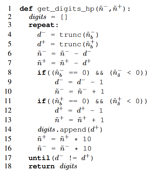
Figure 7: Errol1 algorithm for generating digits based on the boundaries n ˉ − \bar{n}^- nˉ− and n ˉ + \bar{n}^+ nˉ+.
图 7:基于边界 n ˉ − \bar{n}^- nˉ− 与 n ˉ + \bar{n}^+ nˉ+ 的 Errol1 数字生成算法
Truncation in lines 4 and 5 is performed directly on the base component of the boundary. Care must be taken in order to guarantee the accuracy of truncation. Recall that by construction, an H P HP HP value consists of a base component that best approximates the target value (as an F P FP FP) and a smaller offset component that accounts for the remainder (as a non-overlapping F P FP FP). In order for the offset to affect truncation, the base component must be an integer; any non-integer value indicates the H P HP HP value is too far from an integer for the offset component to affect truncation (otherwise the base component is not the best approximation). If the base is an integer, the offset can only affect the truncation if it is negative; the code on lines 8--13 checks and accounts for this case. The extracted digit is removed from the boundary (lines 6, 7, 10, and 13), and the boundary is multiplied by ten (lines 15 and 16) in order to prepare the next digit for extraction. Subtraction is performed on the base component n ^ b \hat{n}_b n^b; the offset is too small to be affected.
第 4--5 行的截断直接在边界的基值分量上执行。必须谨慎处理以保证截断精度。如构造所述, H P HP HP 值由基值分量 (目标值的最优 F P FP FP 近似)与更小的偏移分量 (非重叠 F P FP FP,补足剩余部分)组成。偏移影响截断的前提是基值分量为整数;若非整数,说明 H P HP HP 值离整数较远,偏移分量无法影响截断(否则基值就不是最优近似)。若基值为整数,仅当偏移为负时才会影响截断;第 8--13 行代码检查并处理该情况。从边界中移除提取的数字(第 6、7、10、13 行),边界乘以 10(第 15--16 行),准备提取下一位数字。减法仅在基值分量 n ^ b \hat{n}_b n^b 上执行;偏移极小,不受影响。
Thus, as before, we can show that digits_hp returns a correct and optimal decimal in the given narrow interval:
因此,同前可证 digits_hp 返回给定窄区间内正确且最优的十进制数:
Theorem 3. The function digits_hp ( n ˉ − , n ˉ + ) (\bar{n}^-, \bar{n}^+) (nˉ−,nˉ+) returns the optimal (shortest) decimal value in the interval n ˉ − , n ˉ + \\bar{n}\^-, \\bar{n}\^+ nˉ−,nˉ+.
定理 3 :函数 digits_hp ( n ˉ − , n ˉ + ) (\bar{n}^-, \bar{n}^+) (nˉ−,nˉ+) 返回区间 n ˉ − , n ˉ + \\bar{n}\^-, \\bar{n}\^+ nˉ−,nˉ+ 内最优(最短)的十进制值。
4.4 Double-Double Arithmetic
4.4 双-双精度算术
The eagle-eyed reader will have noticed that Errol1 (i.e. the code in Figures 6 and 7) requires only the following arithmetic operations: (1) add-HP-to-FP (2) multiply-HP-by-FP (3) multiply-HP-by-10 (4) divide-HP-by-10 Next, we describe novel algorithms to implement these arithmetic operations, and provide a detailed error analysis by bounding the maximum error using the standard numerical analysis notion of machine epsilon ϵ \epsilon ϵ (also known as "macheps" or "unit roundoff") 6. In § 4.5, we will use the per-operation error bounds to derive a value for ε that yields Theorem 2. As our H P HP HP format has twice the precision of F P FP FP numbers, our error analysis will be measured in terms of ϵ 2 \epsilon^2 ϵ2 which is equivalent to the maximum round-off error of an H P HP HP number. In the sequel, for all operations, we write x ˉ \bar{x} xˉ and z ˉ \bar{z} zˉ to denote the H P HP HP input and output respectively.
细心读者会发现,Errol1(图 6、7 代码)仅需以下算术运算:(1) H P HP HP 加 F P FP FP;(2) H P HP HP 乘 F P FP FP;(3) H P HP HP 乘 10;(4) H P HP HP 除 10。下文介绍实现这些运算的全新算法,并使用数值分析标准概念机器精度 ϵ \epsilon ϵ(也称 macheps 或单位舍入)6 界定最大误差,给出详细误差分析。§ 4.5 将用单运算误差界推导 ε,证明定理 2。由于 H P HP HP 格式精度是 F P FP FP 的两倍,误差分析以 ϵ 2 \epsilon^2 ϵ2 为单位,等价于 H P HP HP 数的最大舍入误差。后续所有运算中, x ˉ \bar{x} xˉ 表示 H P HP HP 输入, z ˉ \bar{z} zˉ 表示 H P HP HP 输出。
(1) Add-HP-to-FP. In Errol1, we only sum an H P HP HP number x ˉ \bar{x} xˉ with an F P FP FP number y ^ \hat{y} y^ that is smaller than x ˉ \bar{x} xˉ. While not used directly in figures 6 and 7, this procedure serves as a subroutine used in subsequent operations. The output z ˉ \bar{z} zˉ is computed componentwise, using a compensation c c c inspired by the Kahan summation algorithm 8:
(1) H P HP HP 加 F P FP FP :Errol1 中仅将 H P HP HP 数 x ˉ \bar{x} xˉ 与小于 x ˉ \bar{x} xˉ 的 F P FP FP 数 y ^ \hat{y} y^ 相加。该运算虽未直接用于图 6、7,但作为子例程被后续运算调用。输出 z ˉ \bar{z} zˉ 按分量计算,使用受卡汉求和算法 8 启发的补偿项 c c c:
z ^ b ≐ f l t ( x ^ b + y ^ ) , c ≐ ( z ^ b − x ^ b ) − y ^ , z ^ δ ≐ f l t ( x ^ δ − c ) \begin{align*} \hat{z}_b &\doteq \mathrm{flt}\left(\hat{x}_b + \hat{y}\right), \\ c &\doteq \left(\hat{z}b - \hat{x}b\right) - \hat{y}, \\ \hat{z}\delta &\doteq \mathrm{flt}\left(\hat{x}\delta - c\right) \end{align*} z^bcz^δ≐flt(x^b+y^),≐(z^b−x^b)−y^,≐flt(x^δ−c)
The base component z ^ b \hat{z}_b z^b is the best approximation of the sum between the two F P FP FP numbers x ^ b \hat{x}_b x^b and y ^ \hat{y} y^. The value c c c is a backwards compensation that restores the digits that are "lost" when rounding z ^ b \hat{z}b z^b. Most importantly, the compensation c c c is computed exactly without incurring any rounding error. Then, the compensation is added into the offset x ^ δ \hat{x}\delta x^δ and rounded to the nearest F P FP FP. Figure 8 illustrates how the truncated digits are recovered by the compensation.
基值分量 z ^ b \hat{z}_b z^b 是两个 F P FP FP 数 x ^ b \hat{x}_b x^b 与 y ^ \hat{y} y^ 之和的最优近似。值 c c c 是反向补偿项 ,用于恢复对 z ^ b \hat{z}b z^b 舍入时"丢失"的位。最重要的是,补偿项 c c c 可精确计算 ,无任何舍入误差。随后将补偿项加入偏移 x ^ δ \hat{x}\delta x^δ 并舍入到最近 F P FP FP。图 8 展示了补偿如何恢复截断丢失的位。
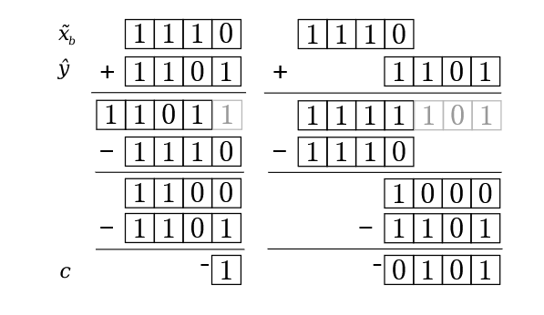
Figure 8: Example of computing the compensation c c c when summing together the F P FP FP numbers x ^ b \hat{x}_b x^b and y ^ \hat{y} y^. The grey numbers correspond to digits that are discarded due to truncation. The left example shows two F P FP FP inputs that are nearly the same size where only a single bit is lost during truncation. The right example shows two inputs of very different size causing truncation of three bits, all of which are recovered.
图 8: F P FP FP 数 x ^ b \hat{x}_b x^b 与 y ^ \hat{y} y^ 相加时补偿项 c c c 的计算示例。灰色数字表示因截断被丢弃的位。左例为两个大小相近的 F P FP FP 输入,截断时仅丢失 1 位;右例为两个大小差异极大的输入,截断时丢失 3 位,但全部被补偿恢复。
Error Analysis. As the compensation c c c recovers all lost bits from the initial summation, the error of the addition operation lies only in the final rounding of x ^ δ − c \hat{x}\delta-c x^δ−c. Thus, due to the non-overlapping invariant, the resulting error is at most ϵ 2 \epsilon^2 ϵ2 for the entire operation.
误差分析 :由于补偿项 c c c 恢复了初始求和中丢失的所有位,加法运算的误差仅来自 x ^ δ − c \hat{x}\delta-c x^δ−c 的最终舍入。因此,在非重叠不变式下,整个运算的误差至多为 ϵ 2 \epsilon^2 ϵ2。
(2) Multiply-HP-by-FP. In Errol1 we need to multiply an H P HP HP number x ˉ \bar{x} xˉ with an F P FP FP number y ^ \hat{y} y^ e.g. at line 6 of figure 6. By expanding the definition for H P HP HP, we can write the output z ˉ \bar{z} zˉ as:
(2) H P HP HP 乘 F P FP FP :Errol1 中需要将 H P HP HP 数 x ˉ \bar{x} xˉ 与 F P FP FP 数 y ^ \hat{y} y^ 相乘,例如图 6 第 6 行。展开 H P HP HP 定义,输出 z ˉ \bar{z} zˉ 可写为:
z ˉ ≐ x ˉ × y ^ = ( x ^ b + x ^ δ ) × y ^ = x ^ b × y ^ + x ^ δ × y ^ \begin{aligned} \bar{z} & \doteq \bar{x} \times \hat{y}=\left(\hat{x}b+\hat{x}\delta\right) \times \hat{y} \\ & =\hat{x}b \times \hat{y}+\hat{x}\delta \times \hat{y} \end{aligned} zˉ≐xˉ×y^=(x^b+x^δ)×y^=x^b×y^+x^δ×y^
The first multiplication is done using Knuth's method of splitting each p p p-bit F P FP FP number into two p 2 \frac{p}{2} 2p-bit F P FP FP numbers and performing long-form multiplication, yielding an H P HP HP result without error 9
第一次乘法使用高德纳方法:将每个 p p p 位 F P FP FP 数拆分为两个 p 2 \frac{p}{2} 2p 位 F P FP FP 数,执行长乘法,无误差地得到 H P HP HP 结果 9:
t ˉ ≐ x ^ b × y ^ \bar{t} \doteq \hat{x}_b \times \hat{y} tˉ≐x^b×y^
Though the second term x ^ δ × y ^ \hat{x}_\delta \times \hat{y} x^δ×y^ can be also computed as an H P HP HP number, we can safely ignore the least-significant F P FP FP (i.e. the offset component), as this portion would almost entirely be lost when rounding the final z ˉ \bar{z} zˉ. Finally, the left term (an H P HP HP) and the right term (an F P FP FP) are added together using the previously described addition algorithm. The entire process is illustrated in Figure 9.
虽然第二项 x ^ δ × y ^ \hat{x}_\delta \times \hat{y} x^δ×y^ 也可计算为 H P HP HP 数,但可以安全忽略其最低有效 F P FP FP 位(即偏移分量),因为这部分在对最终 z ˉ \bar{z} zˉ 舍入时几乎会完全丢失。最后,将左项( H P HP HP)与右项( F P FP FP)用前述加法算法相加。整个过程如图 9 所示。
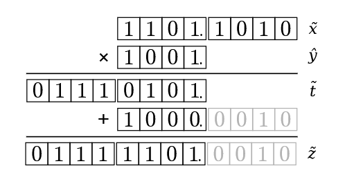
Figure 9: Example: Multiplying a 8-bit H P HP HP number x ˉ \bar{x} xˉ with a 4-bit F P FP FP number y ^ \hat{y} y^. The base x ^ b \hat{x}_b x^b is multiplied by y ^ \hat{y} y^ without error to produce the H P HP HP value t ˉ \bar{t} tˉ. The greyed values are omitted from the computation because they minimally affect the output z ˉ \bar{z} zˉ.
图 9:示例:8 位 H P HP HP 数 x ˉ \bar{x} xˉ 与 4 位 F P FP FP 数 y ^ \hat{y} y^ 相乘。基值 x ^ b \hat{x}_b x^b 与 y ^ \hat{y} y^ 无误差相乘,得到 H P HP HP 值 t ˉ \bar{t} tˉ。灰色值因对输出 z ˉ \bar{z} zˉ 影响极小而被省略。
Error Analysis. There are three possible sources of error: the multiplication of the first term, the multiplication of the second term, and the final summation. The first term x ^ b × y ^ \hat{x}b \times \hat{y} x^b×y^ is computed without error, as explained above. The second term x ^ δ × y ^ \hat{x}\delta \times \hat{y} x^δ×y^ is computed using native F P FP FP multiplication which incurs an error of ϵ \epsilon ϵ. Due to non-overlapping, the components x ^ b \hat{x}b x^b and x ^ δ \hat{x}\delta x^δ must be related by ∣ x ^ b ∣ > ∣ x ^ δ ∣ 2 p − 1 |\hat{x}b|>|\hat{x}\delta| 2^{p-1} ∣x^b∣>∣x^δ∣2p−1, and so:
误差分析 :误差有三个可能来源:第一项乘法、第二项乘法、最终求和。如前所述,第一项 x ^ b × y ^ \hat{x}b \times \hat{y} x^b×y^ 无误差计算。第二项 x ^ δ × y ^ \hat{x}\delta \times \hat{y} x^δ×y^ 使用原生 F P FP FP 乘法计算,引入误差 ϵ \epsilon ϵ。由非重叠不变式,分量 x ^ b \hat{x}b x^b 与 x ^ δ \hat{x}\delta x^δ 满足 ∣ x ^ b ∣ > ∣ x ^ δ ∣ 2 p − 1 |\hat{x}b|>|\hat{x}\delta| 2^{p-1} ∣x^b∣>∣x^δ∣2p−1,因此:
∣ x ^ b y ^ ∣ > ∣ x ^ δ y ^ ∣ 2 p − 1 |\hat{x}b \hat{y}|>|\hat{x}\delta \hat{y}| 2^{p-1} ∣x^by^∣>∣x^δy^∣2p−1
Hence, ∣ x ^ δ y ^ ∣ |\hat{x}\delta \hat{y}| ∣x^δy^∣ is smaller than the final output z ˉ \bar{z} zˉ by a factor of 2 − p + 1 2^{-p+1} 2−p+1 and so the total error caused by the second term is ϵ × 2 − p + 1 \epsilon \times 2^{-p+1} ϵ×2−p+1 or 2 ϵ 2 2\epsilon^2 2ϵ2. Finally, the third source of error, the summation of the H P HP HP value t ˉ \bar{t} tˉ to the unrounded F P FP FP x ^ δ × y ^ \hat{x}\delta \times \hat{y} x^δ×y^, incurs an error of ϵ 2 \epsilon^2 ϵ2 as described above. Thus, in total, the multiply-HP-by-FP has relative error of 3 ϵ 2 3\epsilon^2 3ϵ2.
因此, ∣ x ^ δ y ^ ∣ |\hat{x}\delta \hat{y}| ∣x^δy^∣ 比最终输出 z ˉ \bar{z} zˉ 小 2 − p + 1 2^{-p+1} 2−p+1 倍,第二项带来的总误差为 ϵ × 2 − p + 1 \epsilon \times 2^{-p+1} ϵ×2−p+1,即 2 ϵ 2 2\epsilon^2 2ϵ2。最后,第三个误差来源:将 H P HP HP 值 t ˉ \bar{t} tˉ 与未舍入的 F P FP FP 值 x ^ δ × y ^ \hat{x}\delta \times \hat{y} x^δ×y^ 求和,如前所述引入误差 ϵ 2 \epsilon^2 ϵ2。综上, H P HP HP 乘 F P FP FP 的相对误差总计为 3 ϵ 2 3\epsilon^2 3ϵ2。
( c ) Multiply by 10. The procedure get_digits_hp (Figure 7) frequently uses multiply by 10 to shift the decimal point to the right. Each F P FP FP component (base and offset) is multiplied by 10:
( c ) 乘 10 :过程 get_digits_hp(图 7)频繁使用乘 10 实现小数点右移。每个 F P FP FP 分量(基值与偏移)分别乘以 10:
h ^ ≐ f l t ( 10 × x ^ b ) l ^ ≐ f l t ( 10 × x ^ δ ) \hat{h} \doteq \mathrm{flt}\left(10 \times \hat{x}b\right) \quad \hat{l} \doteq \mathrm{flt}\left(10 \times \hat{x}\delta\right) h^≐flt(10×x^b)l^≐flt(10×x^δ)
Rounding occurs for both operations; though it is tolerable for the lower product l ^ \hat{l} l^, rounding of h ^ \hat{h} h^ incurs a significant amount of error. Fortunately, the product is an addition of some bitshifts, the latter being multiplication by a power of two:
两次运算均会舍入;低位乘积 l ^ \hat{l} l^ 的舍入可容忍,但 h ^ \hat{h} h^ 的舍入会引入显著误差。幸运的是,该乘积可拆分为位移之和,后者是 2 的幂次乘法:
h ^ ≐ 10 × x ^ b = 8 × x ^ b + 2 × x ^ b \hat{h} \doteq 10 \times \hat{x}_b=8 \times \hat{x}_b+2 \times \hat{x}_b h^≐10×x^b=8×x^b+2×x^b
As in add-HP-to-FP, a compensated value c c c is backwards computed to recover the bits lost in the computation of h ^ \hat{h} h^ as an F P FP FP number:
与 H P HP HP 加 F P FP FP 类似,反向计算补偿值 c c c,恢复将 h ^ \hat{h} h^ 计算为 F P FP FP 数时丢失的位:
c ≐ ( h ^ − 8 × x ^ b ) − 2 × x ^ b c \doteq \left(\hat{h}-8 \times \hat{x}_b\right)-2 \times \hat{x}_b c≐(h^−8×x^b)−2×x^b
Note that multiplication by 2 and 8 incurs no error so that the compensated value itself is computed without error. The final output z ˉ \bar{z} zˉ integrates the compensation into the offset component:
注意乘 2 与乘 8 无误差,因此补偿值本身可精确计算。最终输出 z ˉ \bar{z} zˉ 将补偿项并入偏移分量:
z ^ b ≐ h ^ z ^ δ ≐ l ^ − c \hat{z}b \doteq \hat{h} \quad \hat{z}\delta \doteq \hat{l}-c z^b≐h^z^δ≐l^−c
Error Analysis. Multiply-by-10 has three sources of error: computing h ^ \hat{h} h^, computing l ^ \hat{l} l^, and performing the final addition. First, computing h ^ \hat{h} h^ may incur error, but the lost bits are exactly recovered using compensation. Second, the error in l ^ \hat{l} l^ is at most ϵ \epsilon ϵ; when accounting for the size of l ^ \hat{l} l^ compared to z ˉ \bar{z} zˉ, we have at most 2 ϵ 2 2\epsilon^2 2ϵ2 of error. Third, the final addition incurs an additional ϵ 2 \epsilon^2 ϵ2 of error. Combined, multiply-by-10 incurs a maximum relative error of 3 ϵ 2 3\epsilon^2 3ϵ2.
误差分析 :乘 10 有三个误差来源:计算 h ^ \hat{h} h^、计算 l ^ \hat{l} l^、最终加法。第一,计算 h ^ \hat{h} h^ 可能引入误差,但丢失的位通过补偿精确恢复。第二, l ^ \hat{l} l^ 的误差至多为 ϵ \epsilon ϵ;考虑 l ^ \hat{l} l^ 相对于 z ˉ \bar{z} zˉ 的大小,误差至多为 2 ϵ 2 2\epsilon^2 2ϵ2。第三,最终加法额外引入 ϵ 2 \epsilon^2 ϵ2 误差。综上,乘 10 的最大相对误差为 3 ϵ 2 3\epsilon^2 3ϵ2。
(d) Divide-by-10. Division follows a similar pattern to multiplication. First, both components are divided using native F P FP FP numbers:
(d) 除 10 :除法与乘法模式相似。首先,两个分量均用原生 F P FP FP 数做除法:
h ^ ≐ f l t ( x ^ b / 10 ) l ^ ≐ f l t ( x ^ δ / 10 ) \hat{h} \doteq \mathrm{flt}\left(\hat{x}b / 10\right) \quad \hat{l} \doteq \mathrm{flt}\left(\hat{x}\delta / 10\right) h^≐flt(x^b/10)l^≐flt(x^δ/10)
For multiplication, the F P FP FP value h ^ \hat{h} h^ was approximately ten times larger than x ^ b \hat{x}_b x^b; however for division, the base component x ^ b \hat{x}_b x^b is ten times larger. Consequently, we compute the compensated value with respect to the input x ^ b \hat{x}_b x^b (instead of the output):
乘法中 F P FP FP 值 h ^ \hat{h} h^ 约为 x ^ b \hat{x}_b x^b 的 10 倍;而除法中基值分量 x ^ b \hat{x}_b x^b 是 h ^ \hat{h} h^ 的 10 倍。因此,针对输入 x ^ b \hat{x}_b x^b(而非输出)计算补偿值:
c ≐ ( x ^ b − 8 × h ^ ) − 2 × h ^ c \doteq \left(\hat{x}_b-8 \times \hat{h}\right)-2 \times \hat{h} c≐(x^b−8×h^)−2×h^
As with multiplication, the compensation is computed without error. The compensated value c c c corresponds to the backwards difference between the actual and exact results multiplied by ten (i.e. between 10 × h ^ 10 \times \hat{h} 10×h^ and 10 × h ^ 10 \times \hat{h} 10×h^). Notice that the exact error on the output satisfies h ^ − h ^ = c / 10 \hat{h}-\hat{h}=c / 10 h^−h^=c/10. Unfortunately, division often produces numbers of infinite length that cannot be exactly represented by F P FP FP numbers. Consequently, the compensated value is rounded to the nearest F P FP FP value before being integrated into the result z ˉ \bar{z} zˉ:
与乘法一样,补偿值可无误差计算。补偿值 c c c 对应实际结果与精确结果乘以 10 后的反向差值(即 10 × h ^ 10 \times \hat{h} 10×h^ 与真值之间)。注意输出的精确误差满足 h ^ − 真值 = c / 10 \hat{h}-\text{真值}=c / 10 h^−真值=c/10。遗憾的是,除法常产生无限长数字,无法用 F P FP FP 数精确表示。因此,补偿值在并入结果 z ˉ \bar{z} zˉ 前先舍入到最近 F P FP FP 值:
z ^ b ≐ h ^ z ^ δ ≐ l ^ − f l t ( c / 10 ) \hat{z}b \doteq \hat{h} \quad \hat{z}\delta \doteq \hat{l}-\mathrm{flt}(c / 10) z^b≐h^z^δ≐l^−flt(c/10)
Error Analysis. Error occurs during three steps in the division operation: rounding of l ^ \hat{l} l^, rounding of c / 10 c/10 c/10, and error during the final addition. As with the previous operations, rounding l ^ \hat{l} l^ incurs at most 2 ϵ 2 2\epsilon^2 2ϵ2 error, and the final addition incurs ϵ 2 \epsilon^2 ϵ2 error. The rounding of the c / 10 c/10 c/10 term produces an additional error on the order of ϵ 2 \epsilon^2 ϵ2. Combining all sources or error, divide-by-10 has a maximum relative error of 4 ϵ 2 4\epsilon^2 4ϵ2.
误差分析 :除法运算的误差出现在三步: l ^ \hat{l} l^ 的舍入、 c / 10 c/10 c/10 的舍入、最终加法误差。与前述运算一致, l ^ \hat{l} l^ 舍入引入至多 2 ϵ 2 2\epsilon^2 2ϵ2 误差,最终加法引入 ϵ 2 \epsilon^2 ϵ2 误差。 c / 10 c/10 c/10 项舍入额外引入约 ϵ 2 \epsilon^2 ϵ2 误差。所有误差合计,除 10 的最大相对误差为 4 ϵ 2 4\epsilon^2 4ϵ2。
4.5 Ensuring Correctness under Rounding Errors
4.5 舍入误差下的正确性保证
As shown in Figure 3, the maximum amount of error from the algorithm directly affects the selection of the narrow and wide bounds. The worst-case error for the entire Errol1 algorithm is found by summing the maximum error of every operation based on the worst-case run of the algorithm. We use this error to set ε to a value that ensures that the computed boundaries correctly lie within the actual midpoints.
如图 3 所示,算法的最大误差直接影响窄边界与宽边界的选取。Errol1 算法整体的最坏误差由算法最坏执行路径上所有运算的最大误差求和得到。我们用该误差设置 ε,确保计算出的边界正确落在真实中点之间。
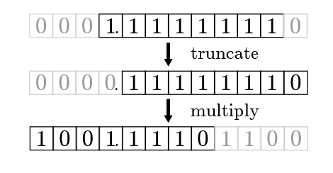
Figure 10: Worst-case error example when generating digits. The dark boxes correspond to an 8-bit floating-point number with a leading 1 bit. Grey boxes correspond to bits that the number cannot represent. Notice that are grey after the multiplication, indicating that they are lost due to truncation.
图 10:数字生成时的最坏误差示例。深色方框表示首位为 1 的 8 位浮点数,灰色方框表示该数无法表示的位。乘法后出现灰色位,表明因截断丢失。
Theorem 4 (Maximum Error). Given an F P FP FP format with a maximum round-off error of ϵ \epsilon ϵ, the maximum relative error of for Errol1 using H P HP HP numbers is at most 79 ϵ 2 79\epsilon^2 79ϵ2.
定理 4(最大误差) :给定最大舍入误差为 ϵ \epsilon ϵ 的 F P FP FP 格式,使用 H P HP HP 数的 Errol1 最大相对误差至多为 79 ϵ 2 79\epsilon^2 79ϵ2。
Proof. From figure 6, there are four loops that are executed a variable number of times. The worst case for small numbers occurs for inputs below 10 − 323 10^{-323} 10−323 where the lookup table can only perform an initial multiply of 10 308 10^{308} 10308. The remaining factor 10 15 10^{15} 1015 requires 15 executions of the loop on lines 10--13 incurring a total error of 45 ϵ 2 45\epsilon^2 45ϵ2. The worst case for large numbers occurs for values above 10 308 10^{308} 10308 where the lookup table can only perform an initial multiply of 10 − 291 10^{-291} 10−291. The remaining factor 10 − 17 10^{-17} 10−17 requires 17 executions of the loop on lines 6--9 incurring a total error of 68 ϵ 2 68\epsilon^2 68ϵ2. Because only a single loop is executed for a given input, the worse case error is the maximum of the two branches 68 ϵ 2 68\epsilon^2 68ϵ2.
证明 :由图 6,有四个循环执行次数可变。小数最坏情况出现在输入小于 10 − 323 10^{-323} 10−323 时,查表仅能执行初始 10 308 10^{308} 10308 乘法,剩余因子 10 15 10^{15} 1015 需要第 10--13 行循环执行 15 次,总误差 45 ϵ 2 45\epsilon^2 45ϵ2。大数最坏情况出现在输入大于 10 308 10^{308} 10308 时,查表仅能执行初始 10 − 291 10^{-291} 10−291 乘法,剩余因子 10 − 17 10^{-17} 10−17 需要第 6--9 行循环执行 17 次,总误差 68 ϵ 2 68\epsilon^2 68ϵ2。由于单个输入仅执行一个循环,最坏误差为两支中的较大值 68 ϵ 2 68\epsilon^2 68ϵ2。
The remaining errors occur in three places: the operations used in exponent computation, a single ϵ 2 \epsilon^2 ϵ2 when computing the powers of ten lookup table, and a loss during digit generation. The digit generation portion of the algorithm loses at most 2 bits of precision (equivalent to 2 ϵ 2 2\epsilon^2 2ϵ2). Future truncation and multiplications do not incur any errors: as digits are extracted, the number of bits shrink such that there is no further rounding. This process, graphically shown in figure 10, demonstrates a worst-case example where an input of all 1 bits is truncated and multiplied by ten to generate a number with two extra bits. Summing all sources of error, the maximum possible error from the entire algorithm is 79 ϵ 2 79\epsilon^2 79ϵ2.
剩余误差出现在三处:指数计算中的运算、10 的幂次查表时的单次 ϵ 2 \epsilon^2 ϵ2、数字生成时的精度损失。数字生成部分最多损失 2 位精度(等价于 2 ϵ 2 2\epsilon^2 2ϵ2)。后续截断与乘法不再引入误差:随着数字被提取,位数减少,不再发生舍入。该过程如图 10 所示,展示了全 1 位输入被截断并乘 10、生成多出 2 位的数的最坏示例。所有误差来源求和,整个算法的最大可能误差为 79 ϵ 2 79\epsilon^2 79ϵ2。
Correctness. Next, we must set the ε to ensure that the bounds on lines 14 and 15 of Figure 6, are indeed correct (i.e. narrow). Setting ε to n ϵ n\epsilon nϵ accounts for n ϵ 2 n\epsilon^2 nϵ2 of error. Thus, for double-precision numbers with ϵ = 2 − 53 \epsilon=2^{-53} ϵ=2−53, we define ε ≐ 8.78 × 10 − 15 \varepsilon \doteq 8.78 \times 10^{-15} ε≐8.78×10⁻¹⁵ which lets us ensure correctness, or formally, Theorem 2.
正确性 :接下来必须设置 ε,确保图 6 第 14--15 行的边界确实是正确的(即窄边界)。将 ε 设为 n ϵ n\epsilon nϵ 可覆盖 n ϵ 2 n\epsilon^2 nϵ2 的误差。因此,对于 ϵ = 2 − 53 \epsilon=2^{-53} ϵ=2−53 的双精度数,定义 ε ≐ 8.78 × 10 − 15 \varepsilon \doteq 8.78 \times 10^{-15} ε≐8.78×10⁻¹⁵,从而保证正确性,即形式化的定理 2。
Optimality. Although Errol1 is not guaranteed to produce the shortest output, the narrow intervals provide a close enough approximation to the rounding interval that Errol1 is guaranteed to produce a decimal output with 17 digits or less.
最优性:虽然 Errol1 不保证输出最短,但窄区间对舍入区间的近似足够接近,使得 Errol1 保证输出不超过 17 位十进制数。
Theorem 5. (Maximum Length) The function convert_hp ( v ^ ) (\hat{v}) (v^) returns a decimal value with at most 17 digits.
定理 5(最大长度) :函数 convert_hp ( v ^ ) (\hat{v}) (v^) 返回至多 17 位的十进制值。
We prove this result using the analysis of Matula that provides an upper bound on the length required to uniquely print a number 11. In particular, given a floating-point format with a radix b b b and p p p bits of precision, every number can be uniquely printed in decimal with D = ⌊ p log 10 b ⌋ + 2 D=\lfloor p \log_{10} b \rfloor+2 D=⌊plog10b⌋+2 digits. We can extend Matula's analysis to our setting (with narrow boundaries) to show that for double-precision floating-point numbers, every floating-point number can be correctly converted with no more than D = 17 D=17 D=17 digits.
该结果使用马图拉的分析证明,其给出了唯一输出一个数所需的位数上界 11。具体而言,给定基数为 b b b、精度为 p p p 位的浮点数格式,每个数都可用 D = ⌊ p log 10 b ⌋ + 2 D=\lfloor p \log_{10} b \rfloor+2 D=⌊plog10b⌋+2 位十进制数唯一输出。我们将马图拉的分析扩展到本文(带窄边界)场景,可证明:对于双精度浮点数,每个浮点数都可使用不超过 D = 17 D=17 D=17 位正确转换。
Empirical Evaluation. By empirically running Errol1 on one billion inputs, we observed that all conversions were correct and 99.973% were optimal as compared to Grisu3's 99.5%. Thus, Errol1 is sub-optimal for an order of magnitude fewer inputs than Grisu3.
实验评估:在 10 亿个输入上实测运行 Errol1,观察到所有转换均正确,99.973% 为最优;而 Grisu3 为 99.5%。因此,Errol1 的非最优输入比例比 Grisu3 低一个数量级。
- 浮点数输出 | 一种完全正确的实现方法(3)-CSDN博客
https://blog.csdn.net/u013669912/article/details/159589035