注:本文为 "浮点数运算" 相关译文,机翻未校。
略作重排,如有内容异常,请看原文。
csdn 篇幅所限,分篇连载。
6. Errol3: Always Optimal
6. Errol3:始终最优
A 99.9999999% optimality rate is not bad, but why leave anything to chance? Next, we present the final refinement, Errol3, which guarantees correct and optimal conversion for all inputs.
99.9999999% 的最优率已经不错,但为何要留下任何不确定性?接下来,我们给出最终改进版 Errol3,它保证对所有输入都正确且最优。
Pathological Inputs and Outputs. A pathological input is an F P FP FP value for which the optimal (shortest) decimal is found extremely close to the midpoint (in the uncovered interval) as shown in Figure 1. The decimal output corresponding to a pathological input is called a pathological output. Note that the Maximum Length Theorem 5, implies that for double-precision floating-point arithmetic, pathological outputs have fewer than 17 digits.
病态输入与输出 :病态输入是指最优(最短)十进制数极其靠近中点(在未覆盖区间内)的 F P FP FP 值,如图 1 所示。与病态输入对应的十进制输出称为病态输出。注意由最大长度定理 5,对双精度浮点运算,病态输出少于 17 位。
Optimality via Enumeration. Errol3 is founded upon two key insights. First, we identify necessary conditions, a set of modular arithmetic constraints, that characterize the midpoints whose neighborhoods contain pathological inputs and outputs (§ 6.2). Second, we provide an efficient algorithm to efficiently enumerate all the solutions to the modular arithmetic constraints, thereby tabulating all the possible pathological inputs and their corresponding outputs (§ 6.3). Thus, given an arbitrary v ^ \hat{v} v^, Errol3 simply checks if it is one of the pathological inputs and if so, returns its tabulated output. Otherwise, it computes using a modified version of Errol2 (§ 6.4).
通过枚举保证最优 :Errol3 基于两个关键洞察。第一,我们识别出一组模算术约束形式的必要条件 ,刻画邻域内包含病态输入与输出的中点(§ 6.2)。第二,我们提供高效算法枚举模算术约束的所有解,从而制表列出所有可能的病态输入及其对应输出(§ 6.3)。因此,给定任意 v ^ \hat{v} v^,Errol3 只需检查它是否是病态输入之一,如果是,返回表中输出;否则使用改进版 Errol2 计算(§ 6.4)。
6.1 Preliminaries
6.1 预备知识
Our analysis partitions the input space by the (binary) exponent e e e, i.e. into sub-ranges comprising the intervals [ 2 e , 2 e + 1 ) [2^e, 2^{e+1}) [2e,2e+1), which we call the input range of e e e. That is, for a given input range, the exponent e e e is a fixed constant. For double-precision floating-point numbers, there are 4098 possible exponents e e e, including subnormal numbers. Our characterization and enumeration algorithm finds all pathological inputs by iteratively searching all possible exponents. In the sequel, we assume a fixed exponent e e e and its input range, and recall that p p p denotes the number of bits of precision of the given format.
我们的分析按(二进制)指数 e e e 划分输入空间,即划分为区间 [ 2 e , 2 e + 1 ) [2^e, 2^{e+1}) [2e,2e+1) 构成的子范围,我们称之为 e e e 的输入范围。即对给定输入范围,指数 e e e 是固定常数。对于双精度浮点数,包括非规格数在内共有 4098 个可能的指数 e e e。我们的刻画与枚举算法通过迭代搜索所有可能指数找到全部病态输入。下文假设指数 e e e 及其输入范围固定,并回顾 p p p 表示给定格式的精度位数。
Enumerating Inputs & Midpoints. The first number (resp. midpoint) in the input range is named v ^ 0 = 2 e \hat{v}_0=2^e v^0=2e (resp. m ˉ 0 = 2 e + 2 e − p − 1 \bar{m}_0=2^e+2^{e-p-1} mˉ0=2e+2e−p−1.) The spacing between floating-point numbers (resp. midpoints) is exactly 2 e − p 2^{e-p} 2e−p. Therefore, the k t h k^{th} kth number (resp. midpoint) in the input range, where k k k is a natural number less than 2 p 2^p 2p, is v ^ k = 2 e + k × 2 e − p \hat{v}_k=2^e+k \times 2^{e-p} v^k=2e+k×2e−p (resp. m ˉ k = 2 e + 2 e − p − 1 + k 2 e − p \bar{m}_k=2^e+2^{e-p-1}+k 2^{e-p} mˉk=2e+2e−p−1+k2e−p).
枚举输入与中点 :输入范围中的第一个数(对应中点)记为 v ^ 0 = 2 e \hat{v}_0=2^e v^0=2e(对应 m ˉ 0 = 2 e + 2 e − p − 1 \bar{m}_0=2^e+2^{e-p-1} mˉ0=2e+2e−p−1)。浮点数(对应中点)之间的间隔恰好为 2 e − p 2^{e-p} 2e−p。因此,输入范围中第 k k k 个数(对应中点),其中 k k k 是小于 2 p 2^p 2p 的自然数,为 v ^ k = 2 e + k × 2 e − p \hat{v}_k=2^e+k \times 2^{e-p} v^k=2e+k×2e−p(对应 m ˉ k = 2 e + 2 e − p − 1 + k 2 e − p \bar{m}_k=2^e+2^{e-p-1}+k 2^{e-p} mˉk=2e+2e−p−1+k2e−p)。
Pathological Range. The pathological range denotes an area around the midpoint m ˉ k \bar{m}_k mˉk that may contain pathological inputs as shown in Figure 12. The size of the pathological range is defined by the error factor, and is:
病态范围 :病态范围指中点 m ˉ k \bar{m}_k mˉk 周围可能包含病态输入的区域,如图 12 所示。病态范围的大小由误差因子定义,为:
( m ˉ k − 2 e − p ε , m ˉ k + 2 e − p ε ) \left( \bar{m}_k-2^{e-p} \varepsilon,\ \bar{m}_k+2^{e-p} \varepsilon \right) (mˉk−2e−pε, mˉk+2e−pε)
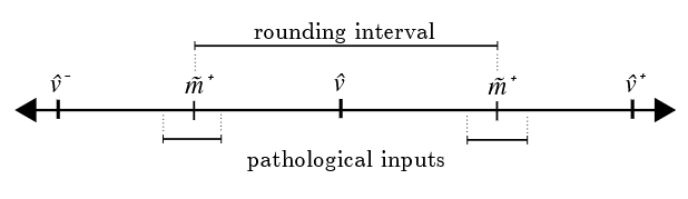
Figure 12: Pathological Input Range. Pathological inputs occur in a small area immediately surrounding the midpoints m ˉ − \bar{m}^- mˉ− and m ˉ + \bar{m}^+ mˉ+.
图 12:病态输入范围。病态输入出现在紧邻中点 m ˉ − \bar{m}^- mˉ− 与 m ˉ + \bar{m}^+ mˉ+ 的小区域内。
Recall that by the Maximum Error Theorem 5, Errol1 has a relative error of at most 79 ϵ 2 79\epsilon^2 79ϵ2. Thus, by setting ε ≥ 79 ϵ \varepsilon \ge 79\epsilon ε≥79ϵ, the pathological range is guaranteed to cover the amount of error incurred by Errol1 (a factor of ϵ \epsilon ϵ is lost from the factor 2 e − p 2^{e-p} 2e−p).
回顾由最大误差定理 5,Errol1 的相对误差至多为 79 ϵ 2 79\epsilon^2 79ϵ2。因此,设置 ε ≥ 79 ϵ \varepsilon \ge 79\epsilon ε≥79ϵ 可保证病态范围覆盖 Errol1 产生的误差(因子 2 e − p 2^{e-p} 2e−p 会损失一个 ϵ \epsilon ϵ 因子)。
Pathological Outputs. A pathological output r r r has the form:
病态输出 :病态输出 r r r 具有形式:
r = m ˉ k + σ 2 e − p = 2 e + 2 e − p − 1 + k 2 e − p + σ 2 e − p = 2 e − p − 1 ( 2 p + 1 + 1 + 2 k + 2 σ ) \begin{aligned} r & =\bar{m}_k+\sigma 2^{e-p}=2^e+2^{e-p-1}+k2^{e-p}+\sigma 2^{e-p} \\ & =2^{e-p-1}(2^{p+1}+1+2k+2\sigma) \end{aligned} r=mˉk+σ2e−p=2e+2e−p−1+k2e−p+σ2e−p=2e−p−1(2p+1+1+2k+2σ)
where ∣ σ ∣ < ε ≤ 79 ϵ |\sigma| < \varepsilon \le 79\epsilon ∣σ∣<ε≤79ϵ
其中 ∣ σ ∣ < ε ≤ 79 ϵ |\sigma| < \varepsilon \le 79\epsilon ∣σ∣<ε≤79ϵ
A value of σ = 0 \sigma=0 σ=0 indicates that r r r is exactly a midpoint. By Theorem 6, outside of the pathological midpoint range, r r r can only be pathological if σ ≠ 0 \sigma \neq 0 σ=0.
σ = 0 \sigma=0 σ=0 表示 r r r 恰好是中点。由定理 6,在病态中点范围之外,仅当 σ ≠ 0 \sigma \neq 0 σ=0 时 r r r 才可能是病态的。
Minimal Congruence. The congruence class z ( m o d n ) z \pmod{n} z(modn) consists of all values v k = z + k n v_k=z+kn vk=z+kn generated by the integers k k k. The minimal congruence, written M c ( z , n ) M_c(z, n) Mc(z,n) is the smallest value from the congruence class z ( m o d n ) z \pmod{n} z(modn). We write M c + ( z , n ) M_c^+(z, n) Mc+(z,n) (resp. M c − ( z , n ) M_c^-(z, n) Mc−(z,n)) for the smallest non-negative (resp. largest non-positive) value from the congruence class z ( m o d n ) z \pmod{n} z(modn).
最小同余 :同余类 z ( m o d n ) z \pmod{n} z(modn) 包含所有由整数 k k k 生成的值 v k = z + k n v_k=z+kn vk=z+kn。最小同余记为 M c ( z , n ) M_c(z, n) Mc(z,n),是同余类 z ( m o d n ) z \pmod{n} z(modn) 中的最小值。我们用 M c + ( z , n ) M_c^+(z, n) Mc+(z,n)(对应 M c − ( z , n ) M_c^-(z, n) Mc−(z,n))表示同余类 z ( m o d n ) z \pmod{n} z(modn) 中最小非负(对应最大非正)值。
6.2 Characterizing Pathologies
6.2 刻画病态性
To characterize pathological inputs and outputs, we partition the input space into those with (i) integer midpoints, i.e. inputs greater than 2 p + 1 2^{p+1} 2p+1, and (ii) non-integer midpoints, i.e. inputs less than 2 p + 1 2^{p+1} 2p+1.
为刻画病态输入与输出,我们将输入空间分为两类:(i) 整数中点,即输入大于 2 p + 1 2^{p+1} 2p+1;(ii) 非整数中点,即输入小于 2 p + 1 2^{p+1} 2p+1。
Integer Midpoints. The following theorem provides a necessary condition that must hold for an integer midpoint m ˉ k > 2 p + 1 \bar{m}_k>2^{p+1} mˉk>2p+1 to have a pathological output r ∗ r^* r∗ in its neighborhood.
整数中点 :下述定理给出一个必要条件:若整数中点 m ˉ k > 2 p + 1 \bar{m}_k>2^{p+1} mˉk>2p+1 的邻域内存在病态输出 r ∗ r^* r∗,则该条件必须成立。
Theorem 7 (Integer Midpoints). A midpoint m ˉ k > 2 p + 1 \bar{m}_k>2^{p+1} mˉk>2p+1, has a pathological output r r r in its neighborhood only if
定理 7(整数中点) :中点 m ˉ k > 2 p + 1 \bar{m}_k>2^{p+1} mˉk>2p+1 的邻域内存在病态输出 r r r 的必要条件为
∣ M c ( m ˉ k , 5 n ) ∣ ≤ ε 2 e − p − n \left| M_c\left( \bar{m}_k, 5^n \right) \right| \le \varepsilon 2^{e-p-n} ∣Mc(mˉk,5n)∣≤ε2e−p−n
where n = ⌊ log 10 r ⌋ − D + 2 n=\left\lfloor \log_{10} r \right\rfloor -D+2 n=⌊log10r⌋−D+2 and m ˉ k = m ˉ k 2 − n \bar{m}_k=\bar{m}_k 2^{-n} mˉk=mˉk2−n
其中 n = ⌊ log 10 r ⌋ − D + 2 n=\left\lfloor \log_{10} r \right\rfloor -D+2 n=⌊log10r⌋−D+2 且 m ˉ k = m ˉ k 2 − n \bar{m}_k=\bar{m}_k 2^{-n} mˉk=mˉk2−n
Proof. First, we show that a pathological output r ∗ r^* r∗ must be an integer. Suppose not, i.e. that r r r is not an integer. Then its right-most index M ( r ) < 0 M(r)<0 M(r)<0 and its left-most index N ( r ) ≥ ⌊ log 10 2 p + 1 ⌋ N(r) \ge \left\lfloor \log_{10} 2^{p+1} \right\rfloor N(r)≥⌊log102p+1⌋. Combined, the length L ( r ) > ⌊ log 10 2 p + 1 ⌋ + 1 L(r)>\left\lfloor \log_{10} 2^{p+1} \right\rfloor +1 L(r)>⌊log102p+1⌋+1. The Maximum Length Theorem 5 implies that such an r r r is too long to be optimal. Therefore, a pathological r r r must be an integer.
证明 :首先证明病态输出 r ∗ r^* r∗ 必为整数。反设 r r r 不是整数,则其最右索引 M ( r ) < 0 M(r)<0 M(r)<0,最左索引 N ( r ) ≥ ⌊ log 10 2 p + 1 ⌋ N(r) \ge \left\lfloor \log_{10} 2^{p+1} \right\rfloor N(r)≥⌊log102p+1⌋。综上,长度 L ( r ) > ⌊ log 10 2 p + 1 ⌋ + 1 L(r)>\left\lfloor \log_{10} 2^{p+1} \right\rfloor +1 L(r)>⌊log102p+1⌋+1。最大长度定理 5 表明这样的 r r r 过长,不可能最优。因此病态 r r r 必为整数。
As done in the analysis of pathological midpoints, we write the length of r r r in terms the left-most index and multiplicities of factors
与病态中点分析相同,我们用最左索引与因子重数表示 r r r 的长度
L ( r ) = ⌊ log 10 r ⌋ − min ( f 5 , f 2 ) + 1 ≤ D − 1 L(r)=\left\lfloor \log_{10} r \right\rfloor -\min(f_5,f_2)+1 \le D-1 L(r)=⌊log10r⌋−min(f5,f2)+1≤D−1
where the latter inequality arises from Theorem 5. Thus, we have a lower bound on the number of prime factors two and five:
后一个不等式由定理 5 得出。因此,我们得到质因子 2 和 5 个数的下界:
min ( f 2 , f 5 ) ≥ ⌊ log 10 r ⌋ − D + 2 \min(f_2,f_5) \ge \lfloor \log_{10} r \rfloor -D+2 min(f2,f5)≥⌊log10r⌋−D+2
Let n n n abbreviate min ( f 2 , f 5 ) \min(f_2,f_5) min(f2,f5). Then r ≡ 0 ( m o d 2 n 5 n ) r \equiv 0 \pmod{2^n 5^n} r≡0(mod2n5n) and so
令 n n n 简写 min ( f 2 , f 5 ) \min(f_2,f_5) min(f2,f5)。则 r ≡ 0 ( m o d 2 n 5 n ) r \equiv 0 \pmod{2^n 5^n} r≡0(mod2n5n),因此
r 2 − n ≡ 0 ( m o d 5 n ) r 2^{-n} \equiv 0 \pmod{5^n} r2−n≡0(mod5n)
Based on the definition of a pathological output, σ \sigma σ is an extremely small, non-zero value. As σ ≪ 1 \sigma \ll 1 σ≪1, σ \sigma σ is not an integer, which implies that r r r cannot divide 2 e − p 2^{e-p} 2e−p. Thus, r r r divides 2 at most e − p − 1 e-p-1 e−p−1 times, or n ≤ e − p − 1 n \le e-p-1 n≤e−p−1. By the midpoint definition, m ˉ k \bar{m}_k mˉk divides 2 e − p − 1 2^{e-p-1} 2e−p−1, and hence, 2 n 2^n 2n. Hence, we create the normalized output r ˉ = r 2 − n \bar{r}=r 2^{-n} rˉ=r2−n and the normalized midpoint m ˉ k = m ˉ k 2 − n \bar{m}_k=\bar{m}_k 2^{-n} mˉk=mˉk2−n related by r ˉ = m ˉ k + σ 2 e − p − n \bar{r}=\bar{m}_k+\sigma 2^{e-p-n} rˉ=mˉk+σ2e−p−n. This lets us write m ˉ k \bar{m}_k mˉk as a congruence class m ˉ k ≡ − σ 2 e − p − n ( m o d 5 n ) \bar{m}_k \equiv -\sigma 2^{e-p-n} \pmod{5^n} mˉk≡−σ2e−p−n(mod5n). As σ \sigma σ is bounded by ε \varepsilon ε (3) there must be a minimal congruence ∣ M c ( m ˉ k , 5 n ) ∣ ≤ ε 2 e − p − n |M_c(\bar{m}_k,5^n)| \le \varepsilon 2^{e-p-n} ∣Mc(mˉk,5n)∣≤ε2e−p−n.
由病态输出定义, σ \sigma σ 是极小非零值。因为 σ ≪ 1 \sigma \ll 1 σ≪1, σ \sigma σ 不是整数,这意味着 r r r 不能整除 2 e − p 2^{e-p} 2e−p。因此, r r r 最多被 2 除 e − p − 1 e-p-1 e−p−1 次,即 n ≤ e − p − 1 n \le e-p-1 n≤e−p−1。由中点定义, m ˉ k \bar{m}_k mˉk 整除 2 e − p − 1 2^{e-p-1} 2e−p−1,因此整除 2 n 2^n 2n。于是我们构造归一化输出 r ˉ = r 2 − n \bar{r}=r 2^{-n} rˉ=r2−n 与归一化中点 m ˉ k = m ˉ k 2 − n \bar{m}_k=\bar{m}_k 2^{-n} mˉk=mˉk2−n,满足 r ˉ = m ˉ k + σ 2 e − p − n \bar{r}=\bar{m}_k+\sigma 2^{e-p-n} rˉ=mˉk+σ2e−p−n。这使我们可将 m ˉ k \bar{m}_k mˉk 写成同余类 m ˉ k ≡ − σ 2 e − p − n ( m o d 5 n ) \bar{m}_k \equiv -\sigma 2^{e-p-n} \pmod{5^n} mˉk≡−σ2e−p−n(mod5n)。由于 σ \sigma σ 受 ε \varepsilon ε(式 3)限制,必存在最小同余 ∣ M c ( m ˉ k , 5 n ) ∣ ≤ ε 2 e − p − n |M_c(\bar{m}_k,5^n)| \le \varepsilon 2^{e-p-n} ∣Mc(mˉk,5n)∣≤ε2e−p−n。
Non-Integer Midpoints. The following theorem provides a necessary condition that must hold for an non-integer midpoint m ˉ k ≤ 2 p + 1 \bar{m}_k \le 2^{p+1} mˉk≤2p+1 to have a pathological output r r r in its neighborhood.
非整数中点 :下述定理给出必要条件:若非整数中点 m ˉ k ≤ 2 p + 1 \bar{m}_k \le 2^{p+1} mˉk≤2p+1 的邻域内存在病态输出 r r r,则该条件必须成立。
Theorem 8 (Non-Integer Range). A midpoint m ˉ k < 2 p + 1 \bar{m}_k<2^{p+1} mˉk<2p+1 has a pathological output r r r in its neighborhood only if
定理 8(非整数范围) :中点 m ˉ k < 2 p + 1 \bar{m}_k<2^{p+1} mˉk<2p+1 的邻域内存在病态输出 r r r 的必要条件为
∣ M c ( m ˉ k , 2 n ) ∣ ≤ ε 5 e − p − n \left| M_c\left( \bar{m}_k, 2^n \right) \right| \le \varepsilon 5^{e-p-n} ∣Mc(mˉk,2n)∣≤ε5e−p−n
where n = ⌊ log 10 r ⌋ − D + 2 n=\left\lfloor \log_{10} r \right\rfloor -D+2 n=⌊log10r⌋−D+2 and m ˉ k = m ˉ k 5 − n 10 − e + p + 1 \bar{m}_k=\bar{m}_k 5^{-n} 10^{-e+p+1} mˉk=mˉk5−n10−e+p+1
其中 n = ⌊ log 10 r ⌋ − D + 2 n=\left\lfloor \log_{10} r \right\rfloor -D+2 n=⌊log10r⌋−D+2 且 m ˉ k = m ˉ k 5 − n 10 − e + p + 1 \bar{m}_k=\bar{m}_k 5^{-n} 10^{-e+p+1} mˉk=mˉk5−n10−e+p+1
Proof. In order to apply the previous integer techniques, the midpoints m ˉ k \bar{m}_k mˉk are scaled by powers of ten to produce integers
证明 :为应用前述整数技术,将中点 m ˉ k \bar{m}_k mˉk 按 10 的幂缩放以生成整数
m ~ k ′ = m ~ k 10 − e + p + 1 = 5 − e + p + 1 2 p + 1 + 5 − e + p + 1 + 2 k 5 − e + p + 1 \begin{aligned} \tilde{m}_k' &= \tilde{m}_k 10^{-e+p+1} \\ &= 5^{-e+p+1} 2^{p+1} + 5^{-e+p+1} + 2k 5^{-e+p+1} \end{aligned} m~k′=m~k10−e+p+1=5−e+p+12p+1+5−e+p+1+2k5−e+p+1
such that m ˉ k ′ ∈ Z \bar{m}_k' \in \mathbb{Z} mˉk′∈Z (shown by applying the Midpoint Format Definition). By construction, their lengths are equal, i.e. L ( m ˉ k ) = L ( m ˉ k ′ ) L(\bar{m}_k)=L(\bar{m}_k') L(mˉk)=L(mˉk′). A pathological output r r r must have the form
使得 m ˉ k ′ ∈ Z \bar{m}_k' \in \mathbb{Z} mˉk′∈Z(由中点格式定义可证)。由构造,它们的长度相等,即 L ( m ˉ k ) = L ( m ˉ k ′ ) L(\bar{m}_k)=L(\bar{m}_k') L(mˉk)=L(mˉk′)。病态输出 r r r 必具有形式
r = 2 e + 2 e − p + k 2 e − p + σ 2 e − p r=2^e+2^{e-p}+k2^{e-p}+\sigma 2^{e-p} r=2e+2e−p+k2e−p+σ2e−p
In order to relate r r r to m ˉ k ′ \bar{m}_k' mˉk′, we construct a modified output r ′ r' r′ as
为将 r r r 与 m ˉ k ′ \bar{m}_k' mˉk′ 关联,我们构造修正输出 r ′ r' r′ 为
r ′ = r 10 − e + p + 1 = m ~ k ′ + 2 σ 5 − e + p = 5 − e + p + 1 2 p + 1 + 5 − e + p + 1 + 2 k 5 − e + p + 1 + 2 σ 5 − e + p = 5 − e + p + 1 ( 2 p + 1 + 1 + 2 k + 2 σ ) \begin{aligned} r' &= r 10^{-e+p+1} \\ &= \tilde{m}_k' + 2\sigma 5^{-e+p} \\ &= 5^{-e+p+1} 2^{p+1} + 5^{-e+p+1} + 2k 5^{-e+p+1} + 2\sigma 5^{-e+p} \\ &= 5^{-e+p+1} \left( 2^{p+1} + 1 + 2k + 2\sigma \right) \end{aligned} r′=r10−e+p+1=m~k′+2σ5−e+p=5−e+p+12p+1+5−e+p+1+2k5−e+p+1+2σ5−e+p=5−e+p+1(2p+1+1+2k+2σ)
so that L ( r ) = L ( r ′ ) L(r)=L(r') L(r)=L(r′). Using the same reasoning as the Integer Range Theorem, we conclude that r ′ r' r′ must be an integer.
使得 L ( r ) = L ( r ′ ) L(r)=L(r') L(r)=L(r′)。使用与整数范围定理相同的推理,可得 r ′ r' r′ 必为整数。
Following the same logic as the previous section by substituting the modified output r ′ r' r′ for the original r r r, we obtain the relation
用修正输出 r ′ r' r′ 替换原始 r r r,遵循与上节相同逻辑,得到关系
min ( f 2 , f 5 ) ≥ ⌊ log 10 r ′ ⌋ − D + 2 \min(f_2,f_5) \ge \left\lfloor \log_{10} r' \right\rfloor -D+2 min(f2,f5)≥⌊log10r′⌋−D+2
Again, we use the name n n n for the minimum number of factors of two and five, and obtain the congruence relations
再次用 n n n 表示因子 2 和 5 的最小个数,得到同余关系
r ′ ≡ 0 ( m o d 2 n 5 n ) ⇒ r ′ 2 − n ≡ 0 ( m o d 5 n ) r' \equiv 0 \pmod{2^n 5^n} \Rightarrow r' 2^{-n} \equiv 0 \pmod{5^n} r′≡0(mod2n5n)⇒r′2−n≡0(mod5n)
By construction, 5 n 5^n 5n must divide r ′ r' r′. Because σ \sigma σ is neither zero nor an integer, r ′ r' r′ cannot divide 5 − e + p + 1 5^{-e+p+1} 5−e+p+1 implying n < − e + p + 1 n<-e+p+1 n<−e+p+1. Because m ˉ k ′ \bar{m}_k' mˉk′ divides 5 − e + p + 1 5^{-e+p+1} 5−e+p+1, it must also divide 5 n 5^n 5n. This fact serves as the basis for creating the normalized output r ˉ = r ′ 5 − n \bar{r}=r' 5^{-n} rˉ=r′5−n and the normalized midpoint m ˉ k = m ˉ k ′ 5 − n \bar{m}_k=\bar{m}_k' 5^{-n} mˉk=mˉk′5−n which are related by:
由构造, 5 n 5^n 5n 必整除 r ′ r' r′。因为 σ \sigma σ 非零且非整数, r ′ r' r′ 不能整除 5 − e + p + 1 5^{-e+p+1} 5−e+p+1,这意味着 n < − e + p + 1 n<-e+p+1 n<−e+p+1。因为 m ˉ k ′ \bar{m}_k' mˉk′ 整除 5 − e + p + 1 5^{-e+p+1} 5−e+p+1,所以它也必整除 5 n 5^n 5n。这一事实是构造归一化输出 r ˉ = r ′ 5 − n \bar{r}=r' 5^{-n} rˉ=r′5−n 与归一化中点 m ˉ k = m ˉ k ′ 5 − n \bar{m}_k=\bar{m}_k' 5^{-n} mˉk=mˉk′5−n 的基础,二者满足:
r ˉ = m ˉ k + σ 5 − e + p − n \bar{r}=\bar{m}_k+\sigma 5^{-e+p-n} rˉ=mˉk+σ5−e+p−n
This previous equation allows us to write m ˉ k \bar{m}_k mˉk as a congruence class
上式使我们可将 m ˉ k \bar{m}_k mˉk 写成同余类
m ˉ k ≡ σ 5 − e + p − n ( m o d 2 n ) \bar{m}_k \equiv \sigma 5^{-e+p-n} \pmod{2^n} mˉk≡σ5−e+p−n(mod2n)
As the value of σ \sigma σ is bounded in terms of ε \varepsilon ε, there must be a minimal congruence such that: ∣ M c ( m ˉ k , 2 n ) ∣ ≤ ε 5 − e + p − n |M_c(\bar{m}_k,2^n)| \le \varepsilon 5^{-e+p-n} ∣Mc(mˉk,2n)∣≤ε5−e+p−n
由于 σ \sigma σ 的值受 ε \varepsilon ε 限制,必存在最小同余使得: ∣ M c ( m ˉ k , 2 n ) ∣ ≤ ε 5 − e + p − n |M_c(\bar{m}_k,2^n)| \le \varepsilon 5^{-e+p-n} ∣Mc(mˉk,2n)∣≤ε5−e+p−n
6.3 Enumerating Pathologies
6.3 枚举病态情况
Theorems 7 and 8 provide necessary conditions for a midpoint m ˉ \bar{m} mˉ to have a pathological output in its interval. Consequently we can phrase the problem of enumerating pathological inputs as computing the solutions of a system of pathological constraints.
定理 7 与 8 给出了中点 m ˉ \bar{m} mˉ 的区间内存在病态输出的必要条件。因此,我们可将枚举病态输入的问题表述为求解病态约束系统。
The Pathological Constraint Problem. Given (1) an arithmetic sequence < m 0 , m 1 , ⋯ > <m_0, m_1, \dots> <m0,m1,⋯> whose k t h k^{th} kth element defined by an initial (normalized midpoint) m 0 m_0 m0 and spacing factor α \alpha α such that m k ≐ m 0 + k × α m_k \doteq m_0+k \times \alpha mk≐m0+k×α; (2) a modulus τ \tau τ; (3) and a threshold Δ \Delta Δ the pathological constraint problem is to compute the set of points m k m_k mk such that ∣ M c ( m k , τ ) ∣ ≤ Δ |M_c(m_k,\tau)| \le \Delta ∣Mc(mk,τ)∣≤Δ
病态约束问题 :给定 (1) 等差数列 < m 0 , m 1 , ⋯ > <m_0, m_1, \dots> <m0,m1,⋯>,其第 k k k 项由初始(归一化中点) m 0 m_0 m0 与间隔因子 α \alpha α 定义,满足 m k ≐ m 0 + k × α m_k \doteq m_0+k \times \alpha mk≐m0+k×α;(2) 模数 τ \tau τ;(3) 阈值 Δ \Delta Δ;病态约束问题是计算满足 ∣ M c ( m k , τ ) ∣ ≤ Δ |M_c(m_k,\tau)| \le \Delta ∣Mc(mk,τ)∣≤Δ 的点集 m k m_k mk。
Exhaustive testing of all midpoints is computationally infeasible for many floating-point formats including double-precision numbers. Instead, we developed an algorithm that finds the (maximal) subsequence of midpoints such that every successive M c ( m k , τ ) M_c(m_k,\tau) Mc(mk,τ) is smaller than the last. In this manner, the algorithm quickly converges on the midpoints that satisfy the pathological constraint.
对包括双精度数在内的许多浮点格式,穷举测试所有中点在计算上不可行。取而代之,我们开发了一种算法,寻找中点的(极大)子序列,使得每个后续的 M c ( m k , τ ) M_c(m_k,\tau) Mc(mk,τ) 都比前一个更小。通过这种方式,算法快速收敛到满足病态约束的中点。
Offsets. An offset is the component of a midpoint that takes the form x k = k α x_k=k\alpha xk=kα. The offset components form a linear relationship where x i + x j = x i + j x_i+x_j=x_{i+j} xi+xj=xi+j. An offset x j x_j xj can be added to a midpoint m i m_i mi to form subsequent midpoints m i + x j = m i + j m_i+x_j=m_{i+j} mi+xj=mi+j. There are two elements of the congruence class m i + j ( m o d τ ) m_{i+j} \pmod{\tau} mi+j(modτ) of importance: the first real number above or equal to z + = M c + ( m i , τ ) z^+=M_c^+(m_i,\tau) z+=Mc+(mi,τ) and the first real number below or equal to z − = M c − ( m i , τ ) z^-=M_c^-(m_i,\tau) z−=Mc−(mi,τ). Based on this interpretation, adding x i x_i xi can be seen as a shift upward to larger real z + z^+ z+ or a shift downward to the smaller real z − z^- z−. For a given offset x j x_j xj, the downward shift and upward shift are respectively defined as:
偏移量 :偏移量是中点的分量,形式为 x k = k α x_k=k\alpha xk=kα。偏移分量满足线性关系 x i + x j = x i + j x_i+x_j=x_{i+j} xi+xj=xi+j。偏移量 x j x_j xj 可加到中点 m i m_i mi 上形成后续中点 m i + x j = m i + j m_i+x_j=m_{i+j} mi+xj=mi+j。同余类 m i + j ( m o d τ ) m_{i+j} \pmod{\tau} mi+j(modτ) 中有两个重要元素:大于等于 z + = M c + ( m i , τ ) z^+=M_c^+(m_i,\tau) z+=Mc+(mi,τ) 的第一个实数,与小于等于 z − = M c − ( m i , τ ) z^-=M_c^-(m_i,\tau) z−=Mc−(mi,τ) 的第一个实数。基于这种解释,加上 x i x_i xi 可视为向上移到更大实数 z + z^+ z+,或向下移到更小实数 z − z^- z−。对给定偏移量 x j x_j xj,向下偏移与向上偏移分别定义为:
x j − ≐ M c − ( x j , τ ) , x j + ≐ M c + ( x j , τ ) x_j^- \doteq M_c^-(x_j,\tau), \quad x_j^+ \doteq M_c^+(x_j,\tau) xj−≐Mc−(xj,τ),xj+≐Mc+(xj,τ)
Using the idea of shifts, the overall goal is restated as: starting at an initial m 0 m_0 m0, find an optimal sequence of shifts that generate successive midpoints closer to zero.
使用偏移思想,整体目标可重述为:从初始 m 0 m_0 m0 开始,寻找最优偏移序列,生成越来越靠近零的连续中点。
Optimal Shift Sequences. The optimal sequence of upward shifts X + X^+ X+ is defined as the lexicographically smallest subsequence of < x 0 + ... x N + > <x_0^+ \dots x_N^+> <x0+...xN+> that is decreasing in magnitude; i.e., for any two adjacent elements x i + , x j + ∈ X + x_i^+, x_j^+ \in X^+ xi+,xj+∈X+, there is no x k + x_k^+ xk+ such that i < k < j i<k<j i<k<j and x i + < x k + < x j + x_i^+<x_k^+<x_j^+ xi+<xk+<xj+. The optimal sequence of downward shifts X − X^- X− is similarly defined with respect to sequence < x 0 − ... x N + > <x_0^- \dots x_N^+> <x0−...xN+>.
最优偏移序列 :向上偏移的最优序列 X + X^+ X+ 定义为 < x 0 + ... x N + > <x_0^+ \dots x_N^+> <x0+...xN+> 中按字典序最小、且幅值严格递减的子序列;即对任意两个相邻元素 x i + , x j + ∈ X + x_i^+, x_j^+ \in X^+ xi+,xj+∈X+,不存在 x k + x_k^+ xk+ 使得 i < k < j i<k<j i<k<j 且 x i + < x k + < x j + x_i^+<x_k^+<x_j^+ xi+<xk+<xj+。向下偏移的最优序列 X − X^- X− 针对序列 < x 0 − ... x N + > <x_0^- \dots x_N^+> <x0−...xN+> 类似定义。
Optimal Sequence Construction. We begin with the initial sequences X 0 + = < x 0 + > X_0^+=<x_0^+> X0+=<x0+> and X 0 − = < x 0 − > X_0^-=<x_0^-> X0−=<x0−>, and by inductively extending them. Without loss of generality, assume j ≤ k j \le k j≤k. Given the two optimal sequences X k − X_k^- Xk− and X j + X_j^+ Xj+, the next element is constructed in the following manner: select the last element x j + ∈ X + x_j^+ \in X^+ xj+∈X+ and select first element x a − ∈ X k − x_a^- \in X_k^- xa−∈Xk− such that x j + + x a − > x k − x_j^++x_a^->x_k^- xj++xa−>xk−; then, the generated element is the sum x z = x j + + x a − x_z=x_j^++x_a^- xz=xj++xa−. This element x z x_z xz represents either a negative shift ( x z ≤ 0 x_z \le 0 xz≤0) or a positive shift ( x z ≥ 0 x_z \ge 0 xz≥0) and is added to the appropriate sequence to create either X z + X_z^+ Xz+ or x z − x_z^- xz−.
最优序列构造 :从初始序列 X 0 + = < x 0 + > X_0^+=<x_0^+> X0+=<x0+> 与 X 0 − = < x 0 − > X_0^-=<x_0^-> X0−=<x0−> 开始,归纳扩展。不失一般性,假设 j ≤ k j \le k j≤k。给定两个最优序列 X k − X_k^- Xk− 与 X j + X_j^+ Xj+,下一个元素按如下方式构造:选取 X + X^+ X+ 中最后一个元素 x j + x_j^+ xj+,并选取 X k − X_k^- Xk− 中第一个满足 x j + + x a − > x k − x_j^++x_a^->x_k^- xj++xa−>xk− 的元素 x a − x_a^- xa−;然后,生成元素为和 x z = x j + + x a − x_z=x_j^++x_a^- xz=xj++xa−。该元素 x z x_z xz 表示负偏移( x z ≤ 0 x_z \le 0 xz≤0)或正偏移( x z ≥ 0 x_z \ge 0 xz≥0),并被加入对应序列以生成 X z + X_z^+ Xz+ 或 x z − x_z^- xz−。
Lemma 2. Given two upward shifts x a + x_a^+ xa+ and x b + x_b^+ xb+, the difference x c = x a + − x b + x_c=x_a^+-x_b^+ xc=xa+−xb+ must be either an upward shift if x c ∈ 0 , τ ) x_c \\in \[0,\\tau) xc∈\[0,τ) and a downward shift if x c ∈ ( − τ , 0 x_c \in (-\tau,0] xc∈(−τ,0]. If x c x_c xc is zero, it is both an upward and downward shift. Symmetrically for two downward shifts x a − x_a^- xa− and x b − x_b^- xb−, their difference must also be either an upward or downward shift or both.
引理 2 :给定两个向上偏移 x a + x_a^+ xa+ 与 x b + x_b^+ xb+,差值 x c = x a + − x b + x_c=x_a^+-x_b^+ xc=xa+−xb+ 若满足 x c ∈ 0 , τ ) x_c \\in \[0,\\tau) xc∈\[0,τ) 必为向上偏移,若满足 x c ∈ ( − τ , 0 x_c \in (-\tau,0] xc∈(−τ,0] 必为向下偏移。若 x c x_c xc 为零,则既是向上也是向下偏移。对两个向下偏移 x a − x_a^- xa− 与 x b − x_b^- xb−,其差值同理必为向上、向下偏移或二者皆是。
Proof. The upward shifts must lie in the range x a + , x b + ∈ [ 0 , τ ) x_a^+, x_b^+ \in [0,\tau) xa+,xb+∈[0,τ), therefore their difference x c x_c xc must lie in the range ( − τ , τ ) (-\tau,\tau) (−τ,τ). Symmetrically, the difference between two downward shifts lie in the same range ( − τ , τ ) (-\tau,\tau) (−τ,τ). The difference x c x_c xc, falling in the range ( − τ , τ ) (-\tau,\tau) (−τ,τ), is either an upward or downward shift or both.
证明 :向上偏移必落在范围 x a + , x b + ∈ [ 0 , τ ) x_a^+, x_b^+ \in [0,\tau) xa+,xb+∈[0,τ) 内,因此其差值 x c x_c xc 必落在 ( − τ , τ ) (-\tau,\tau) (−τ,τ) 内。对称地,两个向下偏移的差值落在相同范围 ( − τ , τ ) (-\tau,\tau) (−τ,τ) 内。落在 ( − τ , τ ) (-\tau,\tau) (−τ,τ) 内的差值 x c x_c xc 必为向上、向下偏移或二者皆是。
Lemma 3. Given natural numbers j j j and c c c such that j < c j<c j<c and shifts x c + x_c^+ xc+ and x j + x_j^+ xj+ such that x c + < x j + x_c^+<x_j^+ xc+<xj+, then there exists a downward shift x c − j − = x c + − x j + x_{c-j}^-=x_c^+-x_j^+ xc−j−=xc+−xj+. Symmetrically, there exists an equivalent upward shift x c − j + = x c − − x j − x_{c-j}^+=x_c^--x_j^- xc−j+=xc−−xj−.
引理 3 :给定自然数 j j j 与 c c c 满足 j < c j<c j<c,偏移 x c + x_c^+ xc+ 与 x j + x_j^+ xj+ 满足 x c + < x j + x_c^+<x_j^+ xc+<xj+,则存在向下偏移 x c − j − = x c + − x j + x_{c-j}^-=x_c^+-x_j^+ xc−j−=xc+−xj+。对称地,存在等价向上偏移 x c − j + = x c − − x j − x_{c-j}^+=x_c^--x_j^- xc−j+=xc−−xj−。
Proof. By Lemma 2, the resulting shift x c − j x_{c-j} xc−j must exist and be either a downward or upward shift. Because x c + < x j + x_c^+<x_j^+ xc+<xj+, the shift x c − j x_{c-j} xc−j must be negative and therefore is a downward shift. The same argument shows that the difference of equivalently defined downward shifts is an upward shift.
证明 :由引理 2,所得偏移 x c − j x_{c-j} xc−j 必存在,且为向下或向上偏移。因为 x c + < x j + x_c^+<x_j^+ xc+<xj+,偏移 x c − j x_{c-j} xc−j 必为负,因此是向下偏移。同理可证等价定义的向下偏移的差值是向上偏移。
Lemma 4. Given an arbitrary shift x c x_c xc that is not found within the optimal sequence of shifts X X X, then there exists an optimal shift x d x_d xd such that d < c d<c d<c and ∣ x d ∣ < ∣ x c ∣ |x_d|<|x_c| ∣xd∣<∣xc∣.
引理 4 :给定任意偏移 x c x_c xc 不在最优偏移序列 X X X 内,则存在最优偏移 x d x_d xd 使得 d < c d<c d<c 且 ∣ x d ∣ < ∣ x c ∣ |x_d|<|x_c| ∣xd∣<∣xc∣。
Proof. Let x d x_d xd be the first element in the optimal sequence X X X that preceeds x c x_c xc. By construction, d < c d<c d<c. Assume ∣ x d ∣ ≥ ∣ x c ∣ |x_d| \ge |x_c| ∣xd∣≥∣xc∣, then x c x_c xc must be an optimal shift and found in X X X, thus reaching a contradiction. Thus, x d x_d xd satisfies the properties of the optimal shift.
证明 :设 x d x_d xd 是最优序列 X X X 中在 x c x_c xc 之前的第一个元素。由构造, d < c d<c d<c。假设 ∣ x d ∣ ≥ ∣ x c ∣ |x_d| \ge |x_c| ∣xd∣≥∣xc∣,则 x c x_c xc 必为最优偏移且在 X X X 中,矛盾。因此 x d x_d xd 满足最优偏移的性质。
Theorem 9. If X k − X_k^- Xk− and X j + X_j^+ Xj+ are optimal subsequences then the inductive extensions X z − X_z^- Xz− or X z + X_z^+ Xz+ are also optimal.
定理 9 :若 X k − X_k^- Xk− 与 X j + X_j^+ Xj+ 是最优子序列,则归纳扩展得到的 X z − X_z^- Xz− 或 X z + X_z^+ Xz+ 也是最优的。
Proof. Without loss of generality, assume x z x_z xz is an upward shift. Assume X z + X_z^+ Xz+ is suboptimal, i.e., there is a x c + x_c^+ xc+ such that j < c < z j<c<z j<c<z and x c + < x j + x_c^+<x_j^+ xc+<xj+. By Lemma 3, there exists a downward shift x c − j − = x c + − x j + x_{c-j}^-=x_c^+-x_j^+ xc−j−=xc+−xj+. Since c < z c<z c<z,the x c − j − x_{c-j}^- xc−j− shift occurs earlier than the selected x z − j − = x a − x_{z-j}^-=x_a^- xz−j−=xa− shift. If x c − j − x_{c-j}^- xc−j− is in X − X^- X−, then the algorithm failed to select the first available downward shift, thus reaching a contradiction. If x c − j − x_{c-j}^- xc−j− is not in x − x^- x−, then by Lemma 4 there exists an optimal shift x p − x_p^- xp− in x − x^- x− that the algorithm failed to select, thus reaching a contradiction.
证明 :不失一般性,假设 x z x_z xz 是向上偏移。假设 X z + X_z^+ Xz+ 非最优,即存在 x c + x_c^+ xc+ 使得 j < c < z j<c<z j<c<z 且 x c + < x j + x_c^+<x_j^+ xc+<xj+。由引理 3,存在向下偏移 x c − j − = x c + − x j + x_{c-j}^-=x_c^+-x_j^+ xc−j−=xc+−xj+。因为 c < z c<z c<z,偏移 x c − j − x_{c-j}^- xc−j− 出现在所选偏移 x z − j − = x a − x_{z-j}^-=x_a^- xz−j−=xa− 之前。若 x c − j − x_{c-j}^- xc−j− 在 X − X^- X− 中,则算法未能选择第一个可用的向下偏移,矛盾。若 x c − j − x_{c-j}^- xc−j− 不在 x − x^- x− 中,则由引理 4,存在最优偏移 x p − x_p^- xp− 在 x − x^- x− 中但算法未选择,矛盾。
Midpoint Search. The midpoint search begins at the initial midpoint m 0 m_0 m0 and is performed inductively. Given a midpoint m k m_k mk that is positive, we select the first offset x i − ∈ X − x_i^- \in X^- xi−∈X− such that the next midpoint m k + i = m k + x i − m_{k+i}=m_k+x_i^- mk+i=mk+xi− is closer to zero ∣ M c ( m k + i , τ ) ∣ < ∣ M ( m k , τ ) ∣ |M_c(m_{k+i},\tau)|<|M(m_k,\tau)| ∣Mc(mk+i,τ)∣<∣M(mk,τ)∣
中点搜索 :中点搜索从初始中点 m 0 m_0 m0 开始,归纳执行。给定正中点 m k m_k mk,我们选择第一个偏移 x i − ∈ X − x_i^- \in X^- xi−∈X− 使得下一个中点 m k + i = m k + x i − m_{k+i}=m_k+x_i^- mk+i=mk+xi− 更靠近零: ∣ M c ( m k + i , τ ) ∣ < ∣ M ( m k , τ ) ∣ |M_c(m_{k+i},\tau)|<|M(m_k,\tau)| ∣Mc(mk+i,τ)∣<∣M(mk,τ)∣
Theorem 10. After the midpoint m k m_k mk, the generated midpoint m k + i m_{k+i} mk+i is the first midpoint whose minimal congruence is closer to zero.
定理 10 :在中点 m k m_k mk 之后,生成的中点 m k + i m_{k+i} mk+i 是第一个最小同余更靠近零的中点。
Proof. By construction, any different shift from X − X^- X− would create a midpoint with too large or small a minimal congruence. Suppose there exists a larger shift x c x_c xc not in x − x^- x− that creates a midpoint satisfying the condition ∣ M c ( m k + c , τ ) ∣ < ∣ M ( m k , τ ) ∣ |M_c(m_{k+c},\tau)|<|M(m_k,\tau)| ∣Mc(mk+c,τ)∣<∣M(mk,τ)∣. Based on this construction, c c c must be larger than i i i (in order to preserve the optimal sequence definition), which indicates that m k + c m_{k+c} mk+c is not the first midpoint closer to zero. By contradiction, the midpoint m k + i m_{k+i} mk+i is the first such midpoint.
证明 :由构造,任何来自 X − X^- X− 的其他偏移都会生成最小同余过大或过小的中点。假设存在更大偏移 x c x_c xc 不在 x − x^- x− 中,生成满足 ∣ M c ( m k + c , τ ) ∣ < ∣ M ( m k , τ ) ∣ |M_c(m_{k+c},\tau)|<|M(m_k,\tau)| ∣Mc(mk+c,τ)∣<∣M(mk,τ)∣ 的中点。由构造, c c c 必大于 i i i(以保持最优序列定义),这表明 m k + c m_{k+c} mk+c 不是第一个更靠近零的中点。矛盾,故 m k + i m_{k+i} mk+i 是第一个这样的中点。
Symmetrically, if m k m_k mk is negative, we select the first offset x i + ∈ X + x_i^+ \in X^+ xi+∈X+ such that the next midpoint is nonpositive. In this manner, we generate a sequence of midpoints that "ping-pong" back and forth across zero, always decreasing in magnitude. In the event that a midpoint satisfying ∣ M ( m k , τ ) ∣ ≤ ε |M(m_k,\tau)| \le \varepsilon ∣M(mk,τ)∣≤ε is found, the above process no longer applies; instead, midpoints are more exhaustively searched by performing all shifts that land within the range − ε , ε -\\varepsilon,\\varepsilon −ε,ε. This ensures that all midpoints satisfying midpoints are found.
对称地,若 m k m_k mk 为负,我们选择第一个偏移 x i + ∈ X + x_i^+ \in X^+ xi+∈X+ 使得下一个中点非正。通过这种方式,我们生成在零两侧"来回弹跳"的中点序列,幅值始终递减。若找到满足 ∣ M ( m k , τ ) ∣ ≤ ε |M(m_k,\tau)| \le \varepsilon ∣M(mk,τ)∣≤ε 的中点,则上述过程不再适用;取而代之,通过执行所有落在 − ε , ε -\\varepsilon,\\varepsilon −ε,ε 范围内的偏移来更彻底地搜索中点。这保证找到所有满足条件的中点。
Handling Subnormals. Because the above has assumed an arbitrary floating-point format with p p p bits of precision, subnormal numbers are easily encoded by modifying the value of p p p based on the exponent e e e. In this manner, the enumeration algorithm searches the subnormal number ranges for pathological inputs.
处理非规格数 :由于上述假设任意精度为 p p p 位的浮点格式,非规格数可通过根据指数 e e e 修改 p p p 值轻松纳入处理。通过这种方式,枚举算法在非规格数范围内搜索病态输入。
6.4 Guaranteeing Optimal Conversion
6.4 保证最优转换
Before running the enumeration algorithm, the underlying algorithm of Errol2 was modified to remove narrowing and widening. Remember, the purpose of narrowing (and widening) is to guarantee the algorithm always generates a correct (or optimal) result. This step is no longer necessary for Errol3 since all suboptimal or incorrect results are enumerated a priori. Hence, Errol3 obtains a performance benefit because verifying outputs at runtime is no longer necessary.
运行枚举算法前,我们修改了 Errol2 的底层算法,移除窄化与宽化步骤。回顾,窄化(与宽化)的目的是保证算法总是生成正确(或最优)结果。对 Errol3 而言,该步骤不再必要,因为所有非最优或错误结果已被预先枚举。因此,Errol3 获得性能优势,因为不再需要运行时验证输出。
After removing the narrowing and widening steps, we used the enumeration algorithm to generate a list of possibly incorrect or suboptimal inputs. Each input was run using Errol2 to enumerate a complete list of inputs that do not generate correct and optimal outputs. In total, we found that only 45 inputs (of the nearly 2 64 2^{64} 264 inputs) generate incorrect or suboptimal results; all other inputs are guaranteed to generete correct and optimal output. In order to correctly and optimally handle the failing inputs, they are hardcoded into a lookup table that maps the failing inputs to correct and optimal outputs. Combining the special handling of integers and this lookup table, Errol3 is guaranteed to be correct and optimal without runtime checks.
移除窄化与宽化步骤后,我们使用枚举算法生成可能错误或非最优的输入列表。对每个输入用 Errol2 运行,枚举所有不生成正确最优输出的输入。总计,我们发现仅 45 个输入(在近 2 64 2^{64} 264 个输入中)生成错误或非最优结果;所有其他输入保证生成正确最优输出。为正确最优地处理失败输入,我们将它们硬编码到查表中,映射失败输入到正确最优输出。结合整数特殊处理与该查表,Errol3 保证无需运行时检查即可正确且最优。
7. Performance Evaluation
7. 性能评估
Next, we evaluate the performance of Errol3 with the goal of comparing it against previous state of the art algorithms.
接下来,我们评估 Errol3 的性能,目标是与现有最优算法对比。
Methodology. Our experiment compares Errol3, Grisu3, and an updated version of Dragon4. For each algorithm, we measure performance by recording the time in clock cycles taken to convert a floating-point representation to a decimal string. Inputs are randomly generated IEEE-754 double-precision floating-point numbers. Outputs consist of a decimal string significand and an integer exponent. All experiments were performed on an Intel® Core™ i7-3667U CPU at 2.00GHz running Xubuntu Linux 14.04 and compiled with gcc 4.8.2. Each algorithm is tested using 20,000 random inputs with each input converted 100 times, of which the median 80 values were averaged to compute the final result. The source code can be downloaded at https://github.com/marcandrysco/Errol. The performance numbers are shown in Figure 13, which we look at part by part.
方法:实验对比 Errol3、Grisu3 与更新版 Dragon4。对每个算法,我们通过记录将浮点表示转换为十进制字符串所需的时钟周期数衡量性能。输入为随机生成的 IEEE-754 双精度浮点数。输出由十进制尾数字符串与整数指数组成。所有实验在 2.00GHz 的 Intel® Core™ i7-3667U CPU、Xubuntu Linux 14.04 系统上运行,使用 gcc 4.8.2 编译。每个算法用 20 000 个随机输入测试,每个输入转换 100 次,取中间 80 个值的平均值作为最终结果。源码可从 https://github.com/marcandrysco/Errol 下载。性能数据如图 13 所示,我们逐部分解读。
Errol3 across all inputs. Figure 13(a) shows the performance of Errol3 in isolation. We can see that its performance across the input space is fairly constant, except for three anomalies. First, Errol3 incurs a slowdown for values larger than 10 291 10^{291} 10291. This is caused by the fact that the lookup table for powers-of-ten can only store numbers down to 10 − 291 10^{-291} 10−291, and so inputs above that point must be normalized by iteratively dividing by ten, incurring a performance penalty. Second, Errol3 incurs two slowdowns for values smaller than 10 − 292 10^{-292} 10−292. This is caused by significant processor slowdowns when operating on subnormal numbers, and the powers-of-ten lookup table can only store numbers down to 10 − 308 10^{-308} 10−308. Finally, there is a sizable performance anomaly for numbers in the range 2 53 2^{53} 253 to 2 131 2^{131} 2131. These are the numbers converted using the integer algorithm which only applies to numbers in that range (§ 5.3).
全输入范围上的 Errol3 :图 13(a) 单独展示 Errol3 的性能。可见其在整个输入空间上性能基本稳定,仅有三处异常。第一,大于 10 291 10^{291} 10291 的数值会变慢,原因是 10 的幂次查表仅能存到 10 − 291 10^{-291} 10−291,超出部分必须循环除以 10 完成归一化,带来性能开销。第二,小于 10 − 292 10^{-292} 10−292 的数值出现两处变慢,原因是非规格数运算会导致处理器明显降速,且 10 的幂次查表仅能存到 10 − 308 10^{-308} 10−308。最后, 2 53 2^{53} 253 到 2 131 2^{131} 2131 范围内的数出现明显性能异常,这些数使用整数算法转换,该算法仅适用于此范围(§ 5.3)。
Errol3 vs. Grisu3. Figure 13(b) compares the performance of Grisu3 (in black) and Errol3 (in grey). Across the entire input space, Errol3 is, on average, 2.4× slower than Grisu3.
Errol3 对比 Grisu3:图 13(b) 对比 Grisu3(黑色)与 Errol3(灰色)的性能。在整个输入空间上,Errol3 平均比 Grisu3 慢 2.4 倍。
Errol3 vs. Dragon4. Figure 13© shows Dragon4 (in black) and Errol3 (in grey). Furthermore, we can also see that the performance of Dragon4 varies significantly across the input space, forming a "V" shape that increases linearly as numbers get further away from 0. In contrast, both Errol3 and Grisu3 have much less variation in performance across the input space. Across the entire input space, Errol3 is, on average, 5.2× faster than Dragon4.
Errol3 对比 Dragon4:图 13© 展示 Dragon4(黑色)与 Errol3(灰色)。可见 Dragon4 的性能在输入空间上波动极大,呈"V"形,数值离 0 越远耗时线性增加。与之相对,Errol3 与 Grisu3 在全输入范围的性能波动小得多。在整个输入空间上,Errol3 平均比 Dragon4 快 5.2 倍。
Errol3 vs Grisu3-with-fallback. Finally, because Grisu3 fails to generate optimal outputs for approximately 0.5% of inputs, we consider a version of Grisu3 which falls back to Dragon4 when Grisu3 fails to generate an optimal output. Figure 13(d) shows this "Grisu3 with fallback" (in black) and Errol3 (in grey). On average, Errol3 is 2.4× slower than Grisu3 with fallback.
Errol3 对比带回退的 Grisu3:最后,由于 Grisu3 在约 0.5% 的输入上无法生成最优输出,我们考虑带回退的 Grisu3 版本:当 Grisu3 无法生成最优输出时回退到 Dragon4。图 13(d) 展示这种"带回退的 Grisu3"(黑色)与 Errol3(灰色)。平均来看,Errol3 比带回退的 Grisu3 慢 2.4 倍。
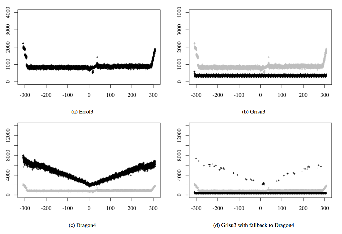
Figure 13 Performance results, shown in black, for (a) Errol3 (b) Grisu3, © Dragon4 and (d) Grisu3 with fallback to Dragon4. Plots (b), ©, and (d) also show Errol3 in grey for reference. Each point plots a single value tested against all algorithms; the x-axis provides the magnitude of the value and the y-axis gives the number of clock cycles required to complete the conversion.
图 13 (a) Errol3、(b) Grisu3、© Dragon4 以及 (d) Grisu3 回退至 Dragon4 的性能结果(以黑色显示)。子图 (b)、© 与 (d) 中同时以灰色显示 Errol3 作为参照。每个数据点表示针对所有算法测试的单一数值;横轴(x 轴)表示数值的量级,纵轴(y 轴)表示完成转换所需的时钟周期数
Performance across Architectures. As Errol3 uses floating-point operations instead of the integer operations used by Grisu3 and Dragon4, its performance compared to those algorithms is dependent on the relative speed of the floating-point operations versus integer operations on a given architecture. Thus, testing Errol3 on a variety of architectures produced an appreciable variation in performance numbers. For example, relative to Dragon4, we observed results ranging from the 5.2× speedup on an Intel® Core™ i7-3667U to a 5.8× on an Intel Xeon X5660.
跨架构性能:由于 Errol3 使用浮点运算,而非 Grisu3 与 Dragon4 所用的整数运算,它与这两种算法的性能对比取决于特定架构上浮点运算与整数运算的相对速度。因此在不同架构上测试 Errol3 会得到明显不同的性能数据。例如,相对于 Dragon4 的加速比:在 Intel® Core™ i7-3667U 上为 5.2 倍,在 Intel Xeon X5660 上为 5.8 倍。
8. Related Work
8. 相关工作
Coonen published an implementation guide for IEEE-754 floating-point arithmetic detailing an early binary-to-decimal conversion algorithm 2, and later expanded on conversion algorithms, covering both correctly rounded and "imperfect" conversions 3.
库宁发表了 IEEE-754 浮点运算实现指南,详细介绍了早期的二进制转十进制算法 2,后续又扩展了转换算法,覆盖正确舍入与"非完美"转换 3。
Steele and White published a paper for printing-floating point numbers that detailed their Dragon4 algorithm 14. Dragon4 provided strong guarantees that the output is both correct and optimal, a process that utilized large integer arithmetic. Later work by Gay 5 and Burger 1 provided performance improvements over the vanilla Dragon4 algorithm.
斯蒂尔与怀特发表浮点数输出论文,详细介绍了 Dragon4 算法 14。Dragon4 提供强保证:输出既正确又最优,该过程使用大整数运算。盖伊 5 与伯格 1 的后续工作在原版 Dragon4 基础上提升了性能。
Loitsch published the Grisu3 algorithm, introducing a fast conversion method that guarantees correct but possibly suboptimal output 10. Unlike previous work, he established a method for verifying the output, and in the 0.05% of cases when the result is suboptimal, the algorithm returns a flag indicating failure. Although Grisu3 significantly outperforms Dragon4 and its successors, Grisu3 still relies on predecessor algorithms as a fallback when it fails to generate optimal outputs.
洛伊奇发表 Grisu3 算法,提出快速转换方法,保证正确但可能非最优的输出 10。与前人工作不同,他建立了输出验证方法,在 0.5% 的非最优情况中,算法返回失败标记。尽管 Grisu3 显著优于 Dragon4 及其改进版,但在无法生成最优输出时,仍依赖前代算法作为回退。
The use of high-precision floating-point data types consisting of multiple, non-overlapping components can be found in previous literature by Knuth 9, Dekker 4, Priest 12, and Shewchuk 13. Previous research by Hida 7 has demonstrated algorithms for supporting a large range of arithmetic operations on floating-point numbers consisting of up to four double-precision numbers.
高德纳 9、德克尔 4、普里斯特 12 与休伊查克 13 的前人文献中已使用由多个非重叠分量组成的高精度浮点数据类型。日高 7 的前期研究展示了支持最多由四个双精度数组成的浮点数的大范围算术运算算法。
Acknowledgements
致谢
We thank the anonymous reviewers for this paper and for a previous version, for their invaluable feedback and suggestions, in particular, for providing a reference to David Matula's In-and-out Conversions 11 which greatly simplified the proof of the Maximum Length Theorem. This work was supported by NSF grant CNS-1514433 and a generous gift from Microsoft Research.
感谢本文与旧版本的匿名审稿人,他们提供了宝贵的反馈与建议,尤其感谢提供大卫·马图拉《双向转换》11 的文献引用,极大简化了最大长度定理的证明。本工作得到美国国家科学基金会基金 CNS-1514433 与微软研究院慷慨捐赠的支持。
References
参考文献
1 R. G. Burger and R. K. Dybvig. Printing floating-point numbers quickly and accurately. In PLDI, 1996.
1 R. G. 伯格,R. K. 迪布维格. 快速精确地输出浮点数. 程序设计语言设计与实现会议(PLDI),1996.
2 J. T. Coonen. An implementation guide to a proposed standard for floating-point arithmetic. IEEE Computer, 13(1), 1980.
2 J. T. 库宁. 浮点运算拟议标准的实现指南. 《IEEE 计算机汇刊》,13(1),1980.
3 J. T. Coonen. Contributions to a Proposed Standard for Binary Floating-point Arithmetic (Computer Arithmetic). PhD thesis, 1984.
3 J. T. 库宁. 二进制浮点运算标准的贡献(计算机运算). 博士论文,1984.
4 T. Dekker. A floating-point technique for extending the available precision. Numerische Mathematik, 18(3), 1971.
4 T. 德克尔. 扩展可用精度的浮点技术. 《数值数学》,18(3),1971.
5 D. M. Gay. Correctly rounded binary-decimal and decimal-binary conversions. In Numerical Analysis Manuscript. 1990.
5 D. M. 盖伊. 正确舍入的二-十与十-二进制转换. 数值分析手稿,1990.
6 D. Goldberg. What every computer scientist should know about floating-point arithmetic. ACM Comput. Surv., 23(1), 1991.
6 D. 戈德堡. 每位计算机科学家都应了解的浮点运算知识. 《ACM 计算调查》,23(1),1991.
7 Y. Hida, X. S. Li, and D. H. Bailey. Algorithms for quad-double precision floating point arithmetic. In Symp. on Computer Arithmetic, 2001.
7 Y. 日高,X. S. 李,D. H. 贝利. 四双精度浮点运算算法. 计算机运算研讨会,2001.
8 W. Kahan. Pracniques: Further remarks on reducing truncation errors. Commun. ACM, 8(1), 1965.
8 W. 卡汉. 实践技巧:关于减少截断误差的补充说明. 《ACM 通讯》,8(1),1965.
9 D. E. Knuth. The Art of Computer Programming, Volume II: Seminumerical Algorithms, 2nd Edition.
9 D. E. 高德纳. 《计算机程序设计艺术》,第二卷:半数值算法,第二版.
10 F. Loitsch. Printing floating-point numbers quickly and accurately with integers. In PLDI, 2010.
10 F. 洛伊奇. 用整数快速精确输出浮点数. 程序设计语言设计与实现会议(PLDI),2010.
11 D. W. Matula. In-and-out conversions. Commun. ACM, 11(1), 1968.
11 D. W. 马图拉. 双向转换. 《ACM 通讯》,11(1),1968.
12 D. M. Priest. On Properties of Floating Point Arithmetics: Numerical Stability and the Cost of Accurate Computations. PhD thesis, 1992.
12 D. M. 普里斯特. 浮点运算的性质:数值稳定性与精确计算的代价. 博士论文,1992.
13 J. R. Shewchuk. Adaptive precision floating-point arithmetic and fast robust geometric predicates. Discrete & Computational Geometry, 18: 305--366, 1996.
13 J. R. 休伊查克. 自适应精度浮点运算与快速鲁棒几何谓词. 《离散与计算几何》,18: 305--366,1996.
14 G. L. Steele and J. L. White. How to print floating-point numbers accurately. In PLDI, 1991.
14 G. L. 斯蒂尔,J. L. 怀特. 如何精确输出浮点数. 程序设计语言设计与实现会议(PLDI),1991.
reference
- fp-printing-popl16.pdf
https://cseweb.ucsd.edu/~lerner/papers/fp-printing-popl16.pdf