第T11周：优化器对比实验

🍨 本文为🔗365天深度学习训练营中的学习记录博客
🍖 原作者：K同学啊

前言

实验环境

python 3.9.2
tensorflow 2.10.0
Jupyter Notebook: 7.4.5

代码实现

设置gpu

python 复制代码

import tensorflow as tf

# 物理GPu列表
gpus = tf.config.list_physical_devices('GPU')

if gpus:
    gpu0 = gpus[0]
    tf.config.experimental.set_memory_growth(gpu0, True)
    tf.config.set_visible_devices(gpus[0], 'GPU') # 确保只用第一张GPU

导入数据

python 复制代码

import warnings
import matplotlib.pyplot as plt
import pathlib

# 忽略警告
warnings.filterwarnings("ignore")
# 解决可视化显示时中文字符可能存在问题
plt.rcParams['font.sans-serif'] = ['SimHei']  # 用来正常显示中文标签
plt.rcParams['axes.unicode_minus'] = False # 用来正常显示负号
# 数据导入
data_dir = "../../datasets/Face"
data_dir = pathlib.Path(data_dir)

image_count = len(list(data_dir.glob('*/*')))

print("图片总数为：{}".format(image_count))

数据加载

python 复制代码

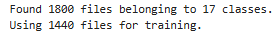
train_ds = tf.keras.preprocessing.image_dataset_from_directory(
    data_dir,
    batch_size= 16, # 每批次处理的图像数量
    image_size=(336, 336), # 自动调整所有图片为该尺寸
    shuffle=True, # 训练集打乱
    seed=123, # 随机种子，确保训练/验证集划分一致
    validation_split=0.2, # 划分 20% 用于验证
    subset="training", # 指定这是训练集
)

python 复制代码

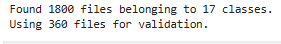
val_ds = tf.keras.preprocessing.image_dataset_from_directory(
    data_dir,
    batch_size= 16, # 每批次处理的图像数量
    image_size=(336, 336), # 自动调整所有图片为该尺寸
    seed=123, # 随机种子，确保训练/验证集划分一致
    validation_split=0.2, # 划分 20% 用于验证
    subset="validation", # 指定这是验证集
)

输出标签

python 复制代码

class_names = train_ds.class_names
print(class_names)

再次检查数据

python 复制代码

for image_batch, labels_batch in train_ds:
    print(image_batch.shape)
    print(labels_batch.shape)
    break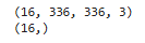

预处理据集以及优化数据加载效率

python 复制代码

AUTOTUNE = tf.data.AUTOTUNE

def train_preprocessing(image,label):
    return (image/255.0,label)

train_ds = (
    train_ds.cache()
    .shuffle(1000)
    .map(train_preprocessing)
    .prefetch(buffer_size=AUTOTUNE)
)

val_ds = (
    val_ds.cache()
    .shuffle(1000)
    .map(train_preprocessing)
    .prefetch(buffer_size=AUTOTUNE)
)

数据可视化

python 复制代码

plt.figure(figsize=(10, 8))  # 图形的宽为10高为5
plt.suptitle("数据展示")

for images, labels in train_ds.take(1):
    for i in range(15):
        plt.subplot(4, 5, i + 1)
        plt.xticks([])
        plt.yticks([])
        plt.grid(False)

        # 显示图片
        plt.imshow(images[i])
        # 显示标签
        plt.xlabel(class_names[labels[i]-1])

plt.show()

构建模型

python 复制代码

from tensorflow.keras.layers import Dropout, Dense, BatchNormalization
from tensorflow.keras.models import Model

batch_size = 16
img_height = 336
img_width = 336

# 定义模型创建函数
def create_model():
    # 加载预训练模型
    vgg16_base_model = tf.keras.applications.vgg16.VGG16(
        weights='imagenet',
        include_top=False,
        input_shape=(img_height, img_width, 3),
        pooling='avg'
    )
    
    # 开启微调，只冻结前一部分层
    vgg16_base_model.trainable = True 
    for layer in vgg16_base_model.layers[:-8]: # 冻结前几个卷积块，解冻最后两个
        layer.trainable = False

    X = vgg16_base_model.output
    X = Dense(170, activation='relu')(X)
    X = BatchNormalization()(X)
    X = Dropout(0.5)(X)

    output = Dense(len(class_names), activation='softmax')(X)
    model = Model(inputs=vgg16_base_model.input, outputs=output)
    
    return model

# 创建三个完全一致的模型实例
model_adam = create_model()   # 用于 Adam (1e-5)
model_sgd_cons = create_model() # 用于 组1：完全一致的 SGD (1e-5, 无动量)
model_sgd_fair = create_model() # 用于 组2：公平对比的 SGD (1e-4, 有动量)

# Adam 配置 (基准) 
model_adam.compile(
    optimizer=tf.keras.optimizers.Adam(learning_rate=1e-5),
    loss='sparse_categorical_crossentropy',
    metrics=['accuracy']
)

# SGD 组1 (绝对一致性控制)
model_sgd_cons.compile(
    optimizer=tf.keras.optimizers.SGD(learning_rate=1e-5), # 不加 momentum
    loss='sparse_categorical_crossentropy',
    metrics=['accuracy']
)

# SGD 组2 (算法潜力公平对比)
model_sgd_fair.compile(
    optimizer=tf.keras.optimizers.SGD(learning_rate=1e-4, momentum=0.9),
    loss='sparse_categorical_crossentropy',
    metrics=['accuracy']
)

model_sgd_fair.summary()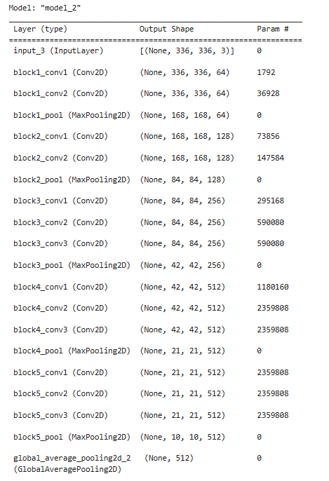

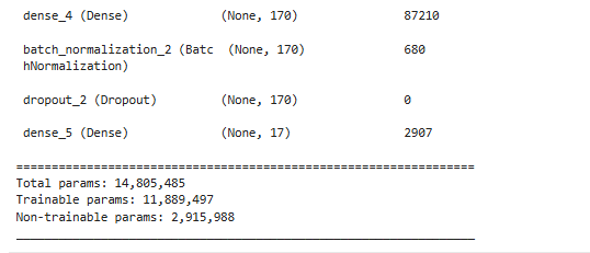
训练模型

python 复制代码

NO_EPOCHS = 20

print("正在训练 Adam (1e-5)...")
history_adam = model_adam.fit(train_ds, epochs=NO_EPOCHS, validation_data=val_ds, verbose=1)

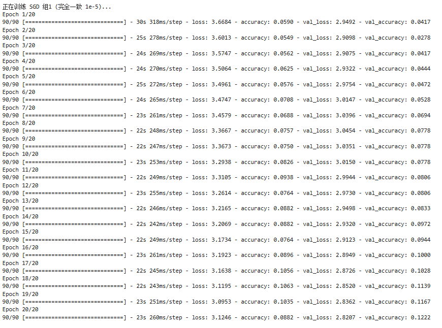
print("\n正在训练 SGD 组1 (完全一致 1e-5)...")
history_sgd_cons = model_sgd_cons.fit(train_ds, epochs=NO_EPOCHS, validation_data=val_ds, verbose=1)

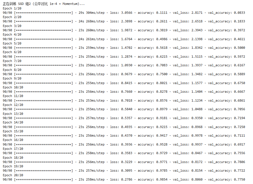
print("\n正在训练 SGD 组2 (公平对比 1e-4 + Momentum)...")
history_sgd_fair = model_sgd_fair.fit(train_ds, epochs=NO_EPOCHS, validation_data=val_ds, verbose=1)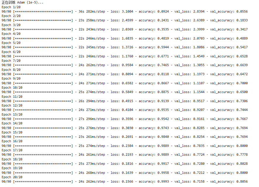

模型评估

图对比

python 复制代码

from matplotlib.ticker import MultipleLocator
import matplotlib.gridspec as gridspec
from datetime import datetime

# 设置绘图参数
plt.rcParams['savefig.dpi'] = 300 
plt.rcParams['figure.dpi']  = 120  # 屏幕显示不用太大
# 设置支持中文的字体
plt.rcParams['font.family'] = ['sans-serif']
plt.rcParams['font.sans-serif'] = ['DejaVu Sans', 'Arial']
current_time = datetime.now().strftime("%Y-%m-%d %H:%M:%S")

# 提取 epoch 长度
epochs_range = range(len(history_adam.history['accuracy']))

# 显著增加高度（10 -> 22），让每个子图都有足够的空间
fig = plt.figure(figsize=(14, 22)) 
gs = gridspec.GridSpec(3, 1, height_ratios=[1, 1, 1], hspace=0.3)

# 统一定义通用刻度定位器（每2轮一个大刻度，更精细）
major_locator = MultipleLocator(2)

# 定义辅助绘图函数，保证风格统一
def plot_learning_curve(ax, history, title_text):
    ax.plot(epochs_range, history['accuracy'], 'b-', linewidth=2.5, label='Train Acc')
    ax.plot(epochs_range, history['val_accuracy'], 'b--', linewidth=2.0, label='Val Acc')
    ax.plot(epochs_range, history['loss'], 'r-', linewidth=2.5, label='Train Loss')
    ax.plot(epochs_range, history['val_loss'], 'r--', linewidth=2.0, label='Val Loss')
    
    ax.set_title(title_text, fontsize=18, fontweight='bold', pad=15)
    ax.set_ylabel('Score / Value', fontsize=14)
    # 底部加上时间戳
    ax.set_xlabel(f'Epochs\n[Logged at: {current_time}]', fontsize=12)
    
    # 放在右下角，设置背景透明度
    legend = ax.legend(loc='lower right', fontsize=11, framealpha=0.8, edgecolor='gray')
    
    # 使用虚线，看起来更高级
    ax.grid(True, linestyle='--', alpha=0.5, color='gray')
    
    # 设置刻度风格
    ax.tick_params(axis='both', which='major', labelsize=11)
    ax.xaxis.set_major_locator(major_locator)
    # y轴刻度微调：0到3.5，间隔0.5
    ax.set_yticks([0, 0.5, 1.0, 1.5, 2.0, 2.5, 3.0, 3.5])

# Adam (1e-5) 基准组 
ax1 = fig.add_subplot(gs[0])

plot_learning_curve(ax1, history_adam.history, '1. Adam (LR=1e-5)\n')

# SGD (1e-5) 绝对一致组
ax2 = fig.add_subplot(gs[1])
# 这里 y 轴刻度由于 Loss 较高，不手动设置yticks，让其自适应显示细节
ax2.set_yticks([]) 
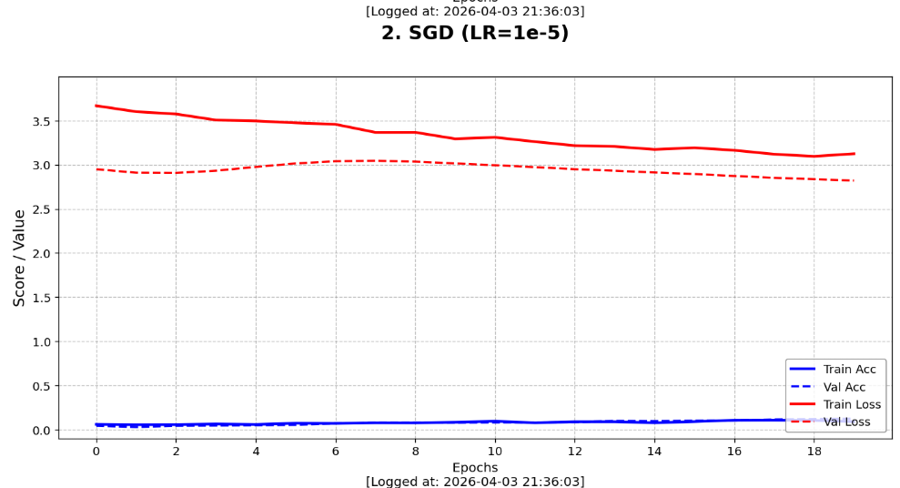
plot_learning_curve(ax2, history_sgd_cons.history, '2. SGD (LR=1e-5)\n')
# 针对组1的 Loss 过高（>3.0），单独微调 y轴
ax2.set_ylim(-0.1, 4.0) 

# SGD (1e-4 + Mom) 公平对比组
ax3 = fig.add_subplot(gs[2])
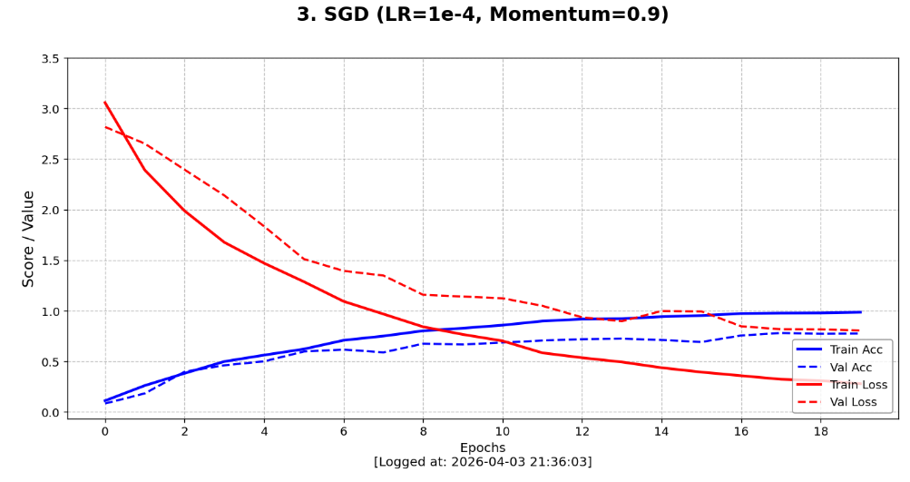
plot_learning_curve(ax3, history_sgd_fair.history, '3. SGD (LR=1e-4, Momentum=0.9)\n')

plt.tight_layout()
plt.show()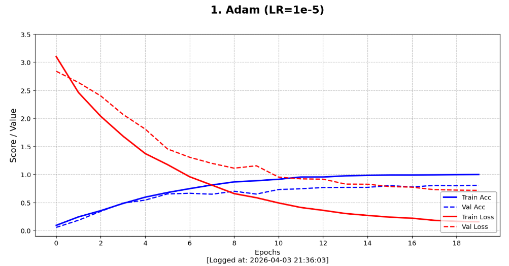

直观对比

python 复制代码

import pandas as pd

def compare_three_models_report(m_adam, m_sgd_cons, m_sgd_fair):
    # 分别评估三个模型
    score_adam = m_adam.evaluate(val_ds, verbose=0)
    score_cons = m_sgd_cons.evaluate(val_ds, verbose=0)
    score_fair = m_sgd_fair.evaluate(val_ds, verbose=0)
    
    # 组织对比数据
    results = {
        '评估指标 (Metric)': ['Loss (损失值)', 'Accuracy (准确率)'],
        'Adam (1e-5)': [f"{score_adam[0]:.4f}", f"{score_adam[1]:.2%}"],
        'SGD 一致组 (1e-5)': [f"{score_cons[0]:.4f}", f"{score_cons[1]:.2%}"],
        'SGD 公平组 (1e-4+Mom)': [f"{score_fair[0]:.4f}", f"{score_fair[1]:.2%}"]
    }
    
    df = pd.DataFrame(results)
    print("三组模型最终评估对比")
    print(df.to_string(index=False))
    
    # 结论输出
    best_acc = max(score_adam[1], score_cons[1], score_fair[1])
    if best_acc == score_adam[1]:
        winner = "Adam (1e-4)"
    elif best_acc == score_fair[1]:
        winner = "SGD 公平对比组"
    else:
        winner = "SGD 一致组"
        
    print(f"表现最优模型：{winner}")

# 调用对比函数
compare_three_models_report(model_adam, model_sgd_cons, model_sgd_fair)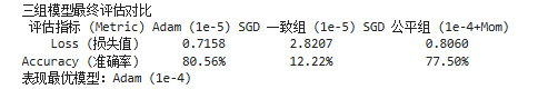

学习总结

我进行了 Adam (1e-5)、SGD 一致组 (1e-5) 与 SGD 公平组 (1e-4 + Momentum) 三个对照模型。
- "SGD 一致组"
  - 设计 SGD (1e-5) 这个组，初衷是为了通过绝对控制变量来观察算法的本性。
  - 收获：实验结果显示，在与 Adam 完全一致的微小步长下，SGD 的准确率曲线几乎没有进步。这让我直观感受到了非自适应优化器的局限性------它缺乏 Adam 那种自动放大梯度的能力。在微调 VGG16 这种深层网络时，如果步长给得不够"狠"，SGD 根本无法跨越损失函数的重重障碍。这有力地反衬了 Adam 在超参设置不精确时，依然能凭借其自适应机制展现出强大的参数容错率和初期爆发力。
- "SGD 公平组"（挖掘算法的真实上限）
  - 如果只看一致组，我会得出"SGD 没法用"的错误结论。因此，我通过引入 100 倍学习率 (1e-4) 并配合 0.9 的动量 (Momentum) 专门设计了"公平对比组"。
  - 收获：这一组的设计是为了观察在各自最佳状态下，传统算法与自适应算法的对比。我发现SGD 组 2 的表现发生了质变。虽然前 5 轮落后于 Adam，但在第 20 轮也稳稳达到了不错的效果
这次实验最大的收获在于我意识到没有绝对"垃圾"的优化器，只有不被理解的参数组合。通过这三个模型的对照，我了解到除了控制变量做对比以外，还有结合优化器特性公平对比看潜力的对比方式。