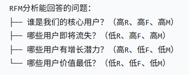
什么是RFM分析:R(Recency)最近一次消费、F(Frequency)、M(Monetary),最近买过、经常买、花得多的用户,是最有价值的用户。
数据集:https://www.kaggle.com/code/ekrembayar/rfm-analysis-online-retail-ii(Kaggle RFM 分析在线零售 II)
一、数据清洗
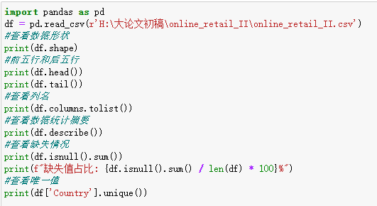
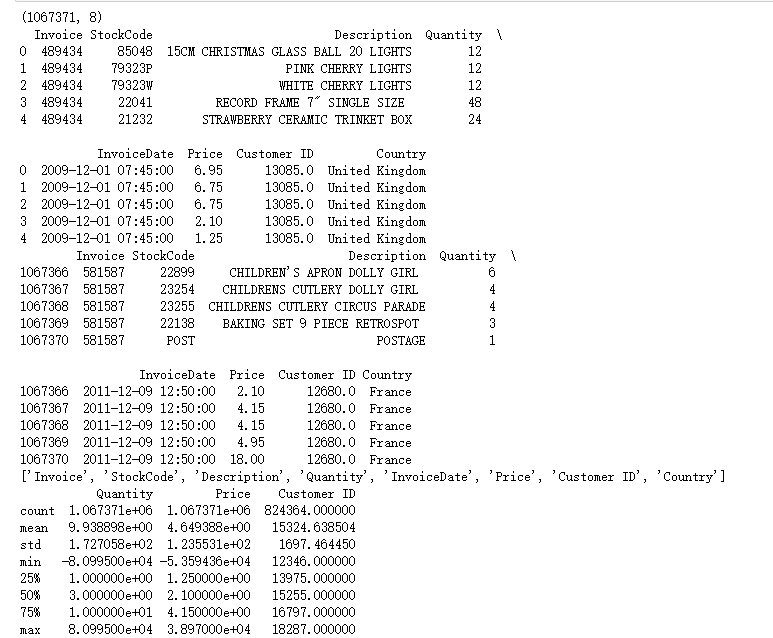
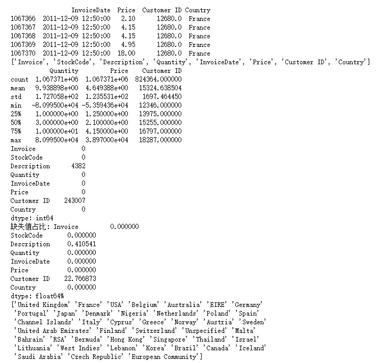
1.初探数据
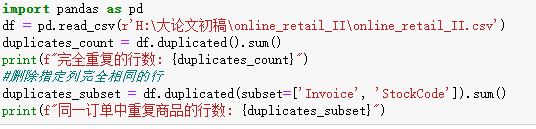
2.处理重复值

3.处理缺失值
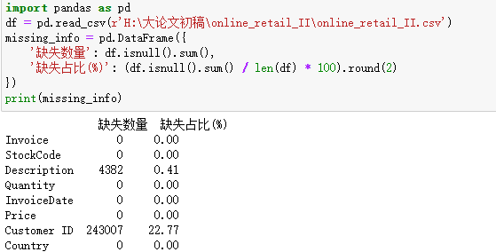
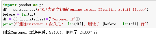
Custmoer ID作为重要的销售信息,缺失占比超过20%,缺失无法做用户分析,将缺失的删除。
Description为描述产品信息的列,不是重要的列,将缺失的内容,统一填充为"Unknown"
df['Description'] = df['Description'].fillna('Unknown')4.处理异常值
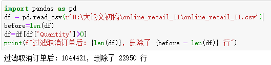
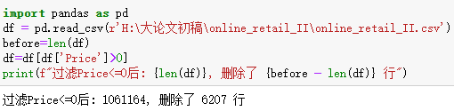
过滤销售数量和销售价格<=0的行
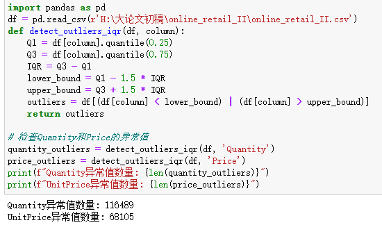
IQR(四分位距法)是数据清洗中常用的异常值识别与剔除方法 ,其核心原理基于数据的四分位数构建合理取值范围。该方法首先计算数据的下四分位数 Q1 与上四分位数 Q3,并通过IQR = Q3 − Q1 得到中间 50% 数据的分布范围;再以Q1 − 1.5×IQR 和Q3 + 1.5×IQR 作为正常数据的上下边界,将超出该范围的数据判定为异常值。IQR 方法基于分位数统计,不受极端值强烈影响,无需假设数据服从正态分布,具有较强的稳健性,适用于各类数值型数据的异常值检测与预处理,是数据分析与预处理中最常用的稳健异常处理手段之一。
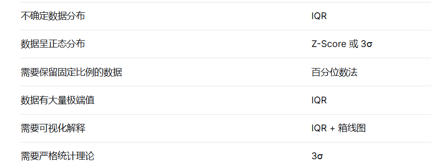
常用的异常值检测的方法:

5.数据转换与特征工程
核心主要为日期处理,目的是将字符串格式的日期转为标准的 datetime 时间类型,以便实现正确的时间排序、筛选、年月季度提取、时间差计算等时间相关分析,同时统一日期格式、消除脏数据带来的分析错误。
df['InvoiceDate'] = pd.to_datetime(df['InvoiceDate'])
df['Date'] = df['InvoiceDate'].dt.date
df['Year'] = df['InvoiceDate'].dt.year
df['Month'] = df['InvoiceDate'].dt.month
df['Day'] = df['InvoiceDate'].dt.day
df['Hour'] = df['InvoiceDate'].dt.hour
df['Weekday'] = df['InvoiceDate'].dt.dayofweek  # 0=周一, 6=周日
df['Weekday_Name'] = df['InvoiceDate'].dt.day_name()
完整的清洗代码:
import pandas as pd
import numpy as np
import warnings
warnings.filterwarnings('ignore')

# ============================================================
# 1. 读取原始数据
# ============================================================

def load_data(file_path):
    """
    加载原始数据
    """
    print("=" * 60)
    print("步骤1:加载数据")
    print("=" * 60)

    df = pd.read_csv(file_path, encoding='latin1')
    print(f"✅ 成功读取CSV文件: {file_path}")
    print(f"原始数据形状: {df.shape}")
    print(f"原始列名: {df.columns.tolist()}")

    return df


# ============================================================
# 2. 数据探索(了解数据质量)
# ============================================================

def explore_data(df):
    """
    探索数据质量
    """
    print("\n" + "=" * 60)
    print("步骤2:数据探索")
    print("=" * 60)

    # 2.1 查看基本信息
    print("\n【2.1 基本信息】")
    print(f"行数: {df.shape[0]:,}")
    print(f"列数: {df.shape[1]}")

    # 2.2 数据类型
    print("\n【2.2 数据类型】")
    print(df.dtypes)

    # 2.3 缺失值统计
    print("\n【2.3 缺失值统计】")
    missing = df.isnull().sum()
    missing_pct = (missing / len(df)) * 100
    missing_df = pd.DataFrame({
        '缺失数量': missing,
        '缺失占比(%)': missing_pct.round(2)
    })
    print(missing_df[missing_df['缺失数量'] > 0])

    # 2.4 重复值统计
    print("\n【2.4 重复值统计】")
    dup_count = df.duplicated().sum()
    print(f"完全重复的行数: {dup_count} ({dup_count/len(df)*100:.2f}%)")

    # 2.5 数值列统计
    print("\n【2.5 数值列统计】")
    numeric_cols = df.select_dtypes(include=[np.number]).columns.tolist()
    if numeric_cols:
        print(df[numeric_cols].describe())

    return df  # 返回原始df,不要返回missing_df


# ============================================================
# 3. 标准化列名(重命名为统一格式)
# ============================================================

def standardize_columns(df):
    """
    标准化列名:重命名为方便使用的格式
    """
    print("\n" + "=" * 60)
    print("步骤3:标准化列名")
    print("=" * 60)

    # 列名映射(原始列名 -> 新列名)
    column_mapping = {
        'Invoice': 'InvoiceNo',
        'StockCode': 'StockCode',
        'Description': 'Description',
        'Quantity': 'Quantity',
        'InvoiceDate': 'InvoiceDate',
        'Price': 'UnitPrice',
        'Customer ID': 'CustomerID',
        'Country': 'Country'
    }

    # 重命名列
    df = df.rename(columns=column_mapping)

    print(f"原始列名: ['Invoice', 'StockCode', 'Description', 'Quantity', 'InvoiceDate', 'Price', 'Customer ID', 'Country']")
    print(f"新列名: {df.columns.tolist()}")

    return df


# ============================================================
# 4. 处理重复值
# ============================================================

def remove_duplicates(df):
    """
    删除完全重复的行
    """
    print("\n" + "=" * 60)
    print("步骤4:处理重复值")
    print("=" * 60)

    before = len(df)
    df = df.drop_duplicates()
    after = len(df)

    print(f"删除前: {before:,} 行")
    print(f"删除后: {after:,} 行")
    print(f"删除了: {before - after:,} 行重复数据")

    return df


# ============================================================
# 5. 处理缺失值
# ============================================================

def handle_missing_values(df):
    """
    处理缺失值
    """
    print("\n" + "=" * 60)
    print("步骤5:处理缺失值")
    print("=" * 60)

    # 5.1 删除 CustomerID 缺失的行(无法做用户分析)
    before = len(df)
    df = df.dropna(subset=['CustomerID'])
    after = len(df)
    print(f"\n【5.1 删除CustomerID缺失】")
    print(f"删除前: {before:,} 行")
    print(f"删除后: {after:,} 行")
    print(f"删除了: {before - after:,} 行 (缺失的CustomerID)")

    # 5.2 填充 Description 缺失
    before_missing = df['Description'].isnull().sum()
    df['Description'] = df['Description'].fillna('Unknown')
    after_missing = df['Description'].isnull().sum()
    print(f"\n【5.2 填充Description缺失】")
    print(f"填充前缺失: {before_missing:,} 行")
    print(f"填充后缺失: {after_missing:,} 行")

    # 5.3 检查其他列的缺失情况
    print(f"\n【5.3 其他列缺失检查】")
    other_missing = df.isnull().sum()
    if other_missing.sum() > 0:
        print(other_missing[other_missing > 0])
    else:
        print("✅ 所有列已无缺失值")

    return df


# ============================================================
# 6. 处理异常值
# ============================================================

def handle_outliers(df):
    """
    处理异常值
    """
    print("\n" + "=" * 60)
    print("步骤6:处理异常值")
    print("=" * 60)

    # 6.1 过滤取消订单(InvoiceNo以C开头)
    before = len(df)
    df = df[~df['InvoiceNo'].astype(str).str.startswith('C')]
    after = len(df)
    print(f"\n【6.1 过滤取消订单】")
    print(f"删除前: {before:,} 行")
    print(f"删除后: {after:,} 行")
    print(f"删除了: {before - after:,} 行取消订单")

    # 6.2 过滤数量 <= 0
    before = len(df)
    df = df[df['Quantity'] > 0]
    after = len(df)
    print(f"\n【6.2 过滤数量<=0】")
    print(f"删除前: {before:,} 行")
    print(f"删除后: {after:,} 行")
    print(f"删除了: {before - after:,} 行")

    # 6.3 过滤单价 <= 0
    before = len(df)
    df = df[df['UnitPrice'] > 0]
    after = len(df)
    print(f"\n【6.3 过滤单价<=0】")
    print(f"删除前: {before:,} 行")
    print(f"删除后: {after:,} 行")
    print(f"删除了: {before - after:,} 行")

    # 6.4 使用IQR方法检测并展示极端异常值(仅展示,不删除)
    print(f"\n【6.4 IQR异常值检测(仅展示,不删除)】")
    for col in ['Quantity', 'UnitPrice']:
        Q1 = df[col].quantile(0.25)
        Q3 = df[col].quantile(0.75)
        IQR = Q3 - Q1
        lower = Q1 - 1.5 * IQR
        upper = Q3 + 1.5 * IQR
        outliers = df[(df[col] < lower) | (df[col] > upper)]
        print(f"  {col}: 检测到 {len(outliers):,} 个异常值 ({len(outliers)/len(df)*100:.2f}%)")
        print(f"    正常范围: [{lower:.2f}, {upper:.2f}]")

    return df


# ============================================================
# 7. 数据类型转换
# ============================================================

def convert_data_types(df):
    """
    转换数据类型
    """
    print("\n" + "=" * 60)
    print("步骤7:数据类型转换")
    print("=" * 60)

    # 7.1 日期转换
    print("\n【7.1 日期转换】")
    df['InvoiceDate'] = pd.to_datetime(df['InvoiceDate'])
    print(f"日期范围: {df['InvoiceDate'].min()} 到 {df['InvoiceDate'].max()}")
    print(f"InvoiceDate 类型: {df['InvoiceDate'].dtype}")

    # 7.2 CustomerID 转换为整数
    print("\n【7.2 CustomerID转换】")
    df['CustomerID'] = df['CustomerID'].astype('Int64')
    print(f"CustomerID 类型: {df['CustomerID'].dtype}")
    print(f"CustomerID 范围: {df['CustomerID'].min()} - {df['CustomerID'].max()}")

    # 7.3 其他类型优化
    print("\n【7.3 其他类型优化】")
    df['Country'] = df['Country'].astype('category')
    print(f"Country 已转换为 category 类型")

    return df


# ============================================================
# 8. 特征工程
# ============================================================

def create_features(df):
    """
    创建新特征
    """
    print("\n" + "=" * 60)
    print("步骤8:特征工程")
    print("=" * 60)

    # 8.1 计算总金额
    df['TotalAmount'] = df['Quantity'] * df['UnitPrice']
    print(f"\n【8.1 总金额】")
    print(f"总金额范围: £{df['TotalAmount'].min():.2f} - £{df['TotalAmount'].max():.2f}")
    print(f"总销售额: £{df['TotalAmount'].sum():,.2f}")
    print(f"平均每笔交易: £{df['TotalAmount'].mean():.2f}")

    # 8.2 提取日期特征
    print(f"\n【8.2 日期特征】")
    df['Year'] = df['InvoiceDate'].dt.year
    df['Month'] = df['InvoiceDate'].dt.month
    df['Day'] = df['InvoiceDate'].dt.day
    df['Hour'] = df['InvoiceDate'].dt.hour
    df['Weekday'] = df['InvoiceDate'].dt.dayofweek
    df['Weekday_Name'] = df['InvoiceDate'].dt.day_name()
    print(f"已添加: Year, Month, Day, Hour, Weekday, Weekday_Name")

    # 8.3 是否周末
    df['IsWeekend'] = df['Weekday'].isin([5, 6]).astype(int)
    print(f"已添加: IsWeekend")

    return df


# ============================================================
# 9. 最终验证与统计
# ============================================================

def final_validation(df):
    """
    最终数据质量验证
    """
    print("\n" + "=" * 60)
    print("步骤9:最终验证")
    print("=" * 60)

    print("\n【9.1 数据概览】")
    print(f"最终数据形状: {df.shape}")
    print(f"用户数: {df['CustomerID'].nunique():,}")
    print(f"订单数: {df['InvoiceNo'].nunique():,}")
    print(f"商品数: {df['StockCode'].nunique():,}")
    print(f"国家数: {df['Country'].nunique():,}")

    print("\n【9.2 缺失值检查】")
    missing = df.isnull().sum()
    if missing.sum() == 0:
        print("✅ 无缺失值")
    else:
        print(missing[missing > 0])

    print("\n【9.3 数据类型检查】")
    print(df.dtypes)

    print("\n【9.4 数值列统计】")
    numeric_cols = df.select_dtypes(include=[np.number]).columns.tolist()
    print(df[numeric_cols].describe())

    print("\n【9.5 国家分布(前10)】")
    print(df['Country'].value_counts().head(10))

    print("\n【9.6 数据时间范围】")
    print(f"最早交易: {df['InvoiceDate'].min()}")
    print(f"最晚交易: {df['InvoiceDate'].max()}")
    print(f"时间跨度: {(df['InvoiceDate'].max() - df['InvoiceDate'].min()).days} 天")

    return df


# ============================================================
# 10. 保存清洗后的数据
# ============================================================

def save_cleaned_data(df, output_path):
    """
    保存清洗后的数据
    """
    print("\n" + "=" * 60)
    print("步骤10:保存数据")
    print("=" * 60)

    # 保存为CSV
    df.to_csv(output_path, index=False)
    print(f"✅ 已保存到: {output_path}")

    return df


# ============================================================
# 主函数:执行完整清洗流程
# ============================================================

def main():
    """
    执行完整的数据清洗流程
    """
    print("\n" + "=" * 60)
    print("数据清洗流程开始")
    print("=" * 60)

    # 文件路径(请修改为你的实际路径)
    input_file = r"H:\大论文初稿\online_retail_II\online_retail_II.csv"
    output_file = r"H:\大论文初稿\online_retail_II\online_retail_II_cleaned.csv"

    # 执行清洗流程
    df = load_data(input_file)
    df = explore_data(df)          # 注意:这里返回df
    df = standardize_columns(df)
    df = remove_duplicates(df)
    df = handle_missing_values(df)
    df = handle_outliers(df)
    df = convert_data_types(df)
    df = create_features(df)
    df = final_validation(df)
    df = save_cleaned_data(df, output_file)

    print("\n" + "=" * 60)
    print("✅ 数据清洗完成!")
    print("=" * 60)

    return df


# ============================================================
# 运行
# ============================================================

if __name__ == "__main__":
    cleaned_df = main()
二、RFM分析
1.计算R、F、M原始值
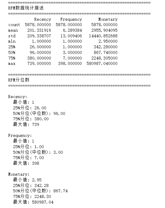
2.查看R、F、M数据分布
3.自定义分箱
使用分位数分箱导致边界和区间数量对不上,改用自定义分箱。
try:
    rfm['R_Score'] = pd.qcut(rfm['Recency'], q=4, labels=[4, 3, 2, 1], duplicates='drop')
    rfm['F_Score'] = pd.qcut(rfm['Frequency'], q=4, labels=[1, 2, 3, 4], duplicates='drop')
    rfm['M_Score'] = pd.qcut(rfm['Monetary'], q=4, labels=[1, 2, 3, 4], duplicates='drop')
    print("✅ 分位数分箱成功")

except ValueError as e:
    print(f"⚠️ 分位数分箱失败: {e}")
    print("切换到自定义分箱...")

    # 自定义分箱
    r_bins = [0, 30, 90, 180, 365]
    r_labels = [4, 3, 2, 1]
    rfm['R_Score'] = pd.cut(rfm['Recency'], bins=r_bins, labels=r_labels, right=False)

    f_bins = [0, 1, 3, 8, 1000]
    f_labels = [1, 2, 3, 4]
    rfm['F_Score'] = pd.cut(rfm['Frequency'], bins=f_bins, labels=f_labels, right=False)

    m_bins = [0, 100, 500, 2000, 100000]
    m_labels = [1, 2, 3, 4]
    rfm['M_Score'] = pd.cut(rfm['Monetary'], bins=m_bins, labels=m_labels, right=False)

    print("✅ 自定义分箱成功")

# 删除缺失值
rfm = rfm.dropna(subset=['R_Score', 'F_Score', 'M_Score'])

# 转换为整数
rfm['R_Score'] = rfm['R_Score'].astype(int)
rfm['F_Score'] = rfm['F_Score'].astype(int)
rfm['M_Score'] = rfm['M_Score'].astype(int)

print(f"\n得分分布:")
print(f"  R_Score: {rfm['R_Score'].value_counts().sort_index().to_dict()}")
print(f"  F_Score: {rfm['F_Score'].value_counts().sort_index().to_dict()}")
print(f"  M_Score: {rfm['M_Score'].value_counts().sort_index().to_dict()}")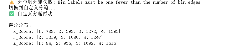
4.GMV分析
GMV:一定时期内所有订单的总金额
单品GMV = 单价 × 数量
# 单个订单的GMV
订单GMV = Σ(该订单中所有商品的 单价 × 数量)
# 总GMV
总GMV = Σ(所有订单的 订单GMV) = Σ(所有商品的 单价 × 数量)
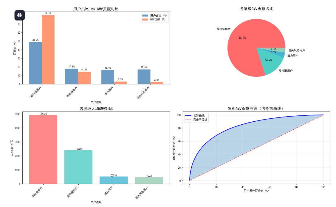
在RFM分析中,GMV贡献用于衡量不同用户层级对总销售额的贡献占比。
# 步骤1:计算各层级的GMV
segment_gmv = rfm.groupby('Segment')['Monetary'].sum()
# 步骤2:计算各层级GMV占比
segment_gmv_ratio = segment_gmv / segment_gmv.sum() * 100
print("各层级GMV贡献:")
for segment, gmv in segment_gmv.items():
ratio = segment_gmv_ratio[segment]
print(f" {segment}: £{gmv:,.2f} ({ratio:.1f}%)")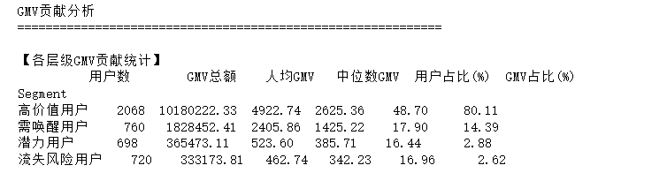 5.完整RFM分析代码
import pandas as pd
import numpy as np
import matplotlib.pyplot as plt
import seaborn as sns
# 设置中文显示
plt.rcParams['font.sans-serif'] = ['SimHei']
plt.rcParams['axes.unicode_minus'] = False
# ============================================================
# 1. 读取清洗后的数据
# ============================================================
df = pd.read_csv(r"H:\大论文初稿\online_retail_II\online_retail_II_cleaned.csv")
# 确保日期格式正确
df['InvoiceDate'] = pd.to_datetime(df['InvoiceDate'])
# 确认列名(应该是 CustomerID,不是 Customer ID)
print("列名列表:", df.columns.tolist())
# ============================================================
# 2. 计算R、F、M原始值
# ============================================================
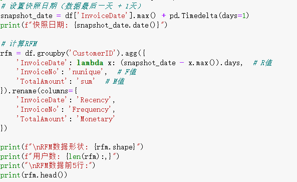
snapshot_date = df['InvoiceDate'].max() + pd.Timedelta(days=1)
print(f"快照日期: {snapshot_date.date()}")
# 使用 CustomerID(注意:没有空格)
rfm = df.groupby('CustomerID').agg({
'InvoiceDate': lambda x: (snapshot_date - x.max()).days, # R值
'InvoiceNo': 'nunique', # F值
'TotalAmount': 'sum' # M值
}).rename(columns={
'InvoiceDate': 'Recency',
'InvoiceNo': 'Frequency',
'TotalAmount': 'Monetary'
})
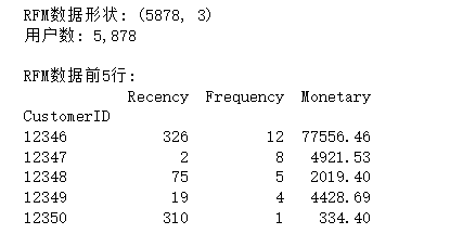
print(f"RFM数据形状: {rfm.shape}")
print(f"用户数: {len(rfm):,}")
# ============================================================
# 3. RFM打分
# ============================================================
try:
rfm['R_Score'] = pd.qcut(rfm['Recency'], q=4, labels=[4, 3, 2, 1], duplicates='drop')
rfm['F_Score'] = pd.qcut(rfm['Frequency'], q=4, labels=[1, 2, 3, 4], duplicates='drop')
rfm['M_Score'] = pd.qcut(rfm['Monetary'], q=4, labels=[1, 2, 3, 4], duplicates='drop')
print("✅ 分位数分箱成功")
except ValueError as e:
print(f"⚠️ 分位数分箱失败: {e}")
print("切换到自定义分箱...")
# 自定义分箱
r_bins = [0, 30, 90, 180, 365]
r_labels = [4, 3, 2, 1]
rfm['R_Score'] = pd.cut(rfm['Recency'], bins=r_bins, labels=r_labels, right=False)
f_bins = [0, 1, 3, 8, 1000]
f_labels = [1, 2, 3, 4]
rfm['F_Score'] = pd.cut(rfm['Frequency'], bins=f_bins, labels=f_labels, right=False)
m_bins = [0, 100, 500, 2000, 100000]
m_labels = [1, 2, 3, 4]
rfm['M_Score'] = pd.cut(rfm['Monetary'], bins=m_bins, labels=m_labels, right=False)
print("✅ 自定义分箱成功")
# 删除缺失值
rfm = rfm.dropna(subset=['R_Score', 'F_Score', 'M_Score'])
# 转换为整数
rfm['R_Score'] = rfm['R_Score'].astype(int)
rfm['F_Score'] = rfm['F_Score'].astype(int)
rfm['M_Score'] = rfm['M_Score'].astype(int)
print(f"\n得分分布:")
print(f" R_Score: {rfm['R_Score'].value_counts().sort_index().to_dict()}")
print(f" F_Score: {rfm['F_Score'].value_counts().sort_index().to_dict()}")
print(f" M_Score: {rfm['M_Score'].value_counts().sort_index().to_dict()}")
# ============================================================
# 4. 用户分层
# ============================================================
def rfm_segment(row):
if row['R_Score'] >= 3 and row['F_Score'] >= 3 and row['M_Score'] >= 3:
return '高价值用户'
elif row['R_Score'] <= 2 and row['F_Score'] >= 3:
return '需唤醒用户'
elif row['R_Score'] >= 3 and row['F_Score'] <= 2:
return '潜力用户'
else:
return '流失风险用户'
rfm['Segment'] = rfm.apply(rfm_segment, axis=1)
# ============================================================
# 5. GMV贡献分析
# ============================================================
print("\n" + "=" * 60)
print("GMV贡献分析")
print("=" * 60)
# 各层级统计
segment_stats = rfm.groupby('Segment').agg({
'Monetary': ['count', 'sum', 'mean', 'median']
}).round(2)
segment_stats.columns = ['用户数', 'GMV总额', '人均GMV', '中位数GMV']
segment_stats = segment_stats.sort_values('GMV总额', ascending=False)
# 计算占比
segment_stats['用户占比(%)'] = (segment_stats['用户数'] / segment_stats['用户数'].sum() * 100).round(2)
segment_stats['GMV占比(%)'] = (segment_stats['GMV总额'] / segment_stats['GMV总额'].sum() * 100).round(2)
print("\n【各层级GMV贡献统计】")
print(segment_stats)
# 贡献倍数
high_value_gmv = segment_stats.loc['高价值用户', '人均GMV'] if '高价值用户' in segment_stats.index else 0
avg_gmv = rfm['Monetary'].mean()
multiplier = high_value_gmv / avg_gmv if avg_gmv > 0 else 0
print(f"\n【贡献分析】")
print(f" 高价值用户人均消费是平均水平的 {multiplier:.1f} 倍")
# 二八定律
top_20_pct = rfm.nlargest(int(len(rfm) * 0.2), 'Monetary')['Monetary'].sum()
top_20_ratio = top_20_pct / rfm['Monetary'].sum() * 100
print(f" 前20%的用户贡献了 {top_20_ratio:.1f}% 的GMV")
# ============================================================
# 6. 可视化
# ============================================================
fig = plt.figure(figsize=(16, 10))
# 图1:用户占比 vs GMV贡献对比
ax1 = fig.add_subplot(2, 2, 1)
segments = segment_stats.index.tolist()
user_pct = segment_stats['用户占比(%)'].values
gmv_pct = segment_stats['GMV占比(%)'].values
x = np.arange(len(segments))
width = 0.35
bars1 = ax1.bar(x - width/2, user_pct, width, label='用户占比 (%)', color='steelblue', alpha=0.8)
bars2 = ax1.bar(x + width/2, gmv_pct, width, label='GMV贡献 (%)', color='coral', alpha=0.8)
ax1.set_xlabel('用户层级')
ax1.set_ylabel('百分比 (%)')
ax1.set_title('用户占比 vs GMV贡献对比', fontsize=14)
ax1.set_xticks(x)
ax1.set_xticklabels(segments, rotation=45, ha='right')
ax1.legend()
for bar, val in zip(bars1, user_pct):
ax1.text(bar.get_x() + bar.get_width()/2, bar.get_height() + 1, f'{val:.1f}%', ha='center', va='bottom', fontsize=9)
for bar, val in zip(bars2, gmv_pct):
ax1.text(bar.get_x() + bar.get_width()/2, bar.get_height() + 1, f'{val:.1f}%', ha='center', va='bottom', fontsize=9)
# 图2:GMV贡献饼图
ax2 = fig.add_subplot(2, 2, 2)
colors = ['#ff6b6b', '#4ecdc4', '#45b7d1', '#96ceb4']
ax2.pie(segment_stats['GMV占比(%)'], labels=segment_stats.index, autopct='%1.1f%%', colors=colors)
ax2.set_title('各层级GMV贡献占比', fontsize=14)
# 图3:人均GMV对比
ax3 = fig.add_subplot(2, 2, 3)
avg_gmv_values = segment_stats['人均GMV']
bars = ax3.bar(segments, avg_gmv_values, color=colors, alpha=0.8)
ax3.set_xlabel('用户层级')
ax3.set_ylabel('人均GMV (£)')
ax3.set_title('各层级人均GMV对比', fontsize=14)
ax3.set_xticklabels(segments, rotation=45, ha='right')
for bar, val in zip(bars, avg_gmv_values):
ax3.text(bar.get_x() + bar.get_width()/2, bar.get_height() + 5, f'£{val:.0f}', ha='center', va='bottom', fontsize=9)
# 图4:累积GMV贡献曲线
ax4 = fig.add_subplot(2, 2, 4)
rfm_sorted = rfm.sort_values('Monetary', ascending=False)
rfm_sorted['cumulative_gmv'] = rfm_sorted['Monetary'].cumsum()
rfm_sorted['cumulative_pct'] = rfm_sorted['cumulative_gmv'] / rfm_sorted['Monetary'].sum() * 100
rfm_sorted['user_pct'] = (np.arange(len(rfm_sorted)) + 1) / len(rfm_sorted) * 100
ax4.plot(rfm_sorted['user_pct'], rfm_sorted['cumulative_pct'], 'b-', linewidth=2, label='实际曲线')
ax4.plot([0, 100], [0, 100], 'r--', linewidth=1, label='完全平等线')
ax4.fill_between(rfm_sorted['user_pct'], rfm_sorted['cumulative_pct'], rfm_sorted['user_pct'], alpha=0.3)
ax4.set_xlabel('用户累计百分比 (%)')
ax4.set_ylabel('GMV累计百分比 (%)')
ax4.set_title('累积GMV贡献曲线(洛伦兹曲线)', fontsize=14)
ax4.legend()
ax4.grid(True, alpha=0.3)
plt.tight_layout()
plt.savefig('GMV_contribution_analysis.png', dpi=150, bbox_inches='tight')
plt.show()
print("\n✅ 图表已保存: GMV_contribution_analysis.png")
# ============================================================
# 7. 业务建议
# ============================================================
print("\n" + "=" * 60)
print("业务建议报告")
print("=" * 60)
for segment in ['高价值用户', '需唤醒用户', '潜力用户', '流失风险用户']:
if segment in segment_stats.index:
seg_data = rfm[rfm['Segment'] == segment]
print(f"\n【{segment}】")
print(f" ├─ 用户数: {len(seg_data):,}人 ({segment_stats.loc[segment, '用户占比(%)']:.1f}%)")
print(f" ├─ GMV贡献: £{seg_data['Monetary'].sum():,.2f} ({segment_stats.loc[segment, 'GMV占比(%)']:.1f}%)")
print(f" ├─ 人均GMV: £{seg_data['Monetary'].mean():.2f}")
print(f" └─ 平均购买次数: {seg_data['Frequency'].mean():.1f}次")
# ============================================================
# 8. 保存结果
# ============================================================
rfm.to_csv('RFM_analysis_complete.csv')
segment_stats.to_csv('GMV_contribution_stats.csv')
print("\n✅ 结果已保存")
print(" - RFM_analysis_complete.csv")
print(" - GMV_contribution_stats.csv")