电离层TEC地图中添加晨昏线/昼夜转换线

在空间天气和电离层研究中，电离层总电子含量（Total Electron Content, TEC）是描述电离层特性的重要参数。TEC地图通常展示全球或区域范围内的电子总密度含量，但电离层的特性在昼夜之间会有显著变化。在TEC地图中添加昼夜转换线（terminator）能够直观地展示日-夜边界，帮助我们理解太阳光照对电离层的影响。

主要用到Cartopy的Nightshade功能

python 复制代码

from cartopy.feature.nightshade import Nightshade
night_shade = Nightshade(target_time, alpha=0.15, edgecolor='none')
ax.add_feature(night_shade)

Cartopy 中的 Nightshade功能是用于在地图上绘制夜晚区域的阴影效果，通常用于可视化全球的昼夜分界线。以下是其主要特性和使用方法：

主要功能

昼夜阴影：根据给定的日期和时间，在地图上绘制出夜晚区域（即太阳照射不到的区域）。
可自定义时间：可以指定具体的日期和时间，计算对应时刻的昼夜分界。
视觉效果：通常以半透明的深色阴影表示夜晚，使地图更具时空感。

完整代码如下：

python 复制代码

# -*- coding: utf-8 -*-
"""
PLOT GIM TEC

@author: OMEGA
"""

import xarray as xr
import numpy as np
import matplotlib.pyplot as plt
import cartopy.crs as ccrs
import cartopy.feature as cfeature
# from cartopy.mpl.gridliner import LONGITUDE_FORMATTER, LATITUDE_FORMATTER
from datetime import datetime
import os
from cartopy.feature.nightshade import Nightshade

plt.rcParams['font.sans-serif'] = ['SimHei', 'Microsoft YaHei', 'DejaVu Sans']
plt.rcParams['axes.unicode_minus'] = False  # 解决负号显示问题
        
def plot_tec_with_contour(nc_file_path, target_time, output_path=None):
    """
    使用等高线方式显示TEC分布
    """
    ds = xr.open_dataset(nc_file_path)
    
    if isinstance(target_time, str):
        target_time = datetime.strptime(target_time, '%Y-%m-%d %H:%M:%S')
    
    tec_data = ds['tec'].sel(time=target_time, method='nearest')
    tec_values = tec_data.values
    actual_time = tec_data.time.values
    
    # 创建图形
    fig = plt.figure(figsize=(16, 9))
    ax = plt.axes(projection=ccrs.PlateCarree())
    
    # 地图要素
    ax.add_feature(cfeature.COASTLINE, linewidth=0.6)
    ax.add_feature(cfeature.BORDERS, linewidth=0.3)
    ax.add_feature(cfeature.OCEAN, color='lightblue', alpha=0.2)
    
    # 经纬度网格
    lon = ds.longitude.values
    lat = ds.latitude.values
    lon_grid, lat_grid = np.meshgrid(lon, lat)
    
    # 绘制等高线
    levels = np.linspace(0, 120, 41)  # 0-50 TECU，分20个等级
    contour = ax.contourf(lon_grid, lat_grid, tec_values, 
                         levels=levels, cmap='jet', 
                         transform=ccrs.PlateCarree(), extend='both')
    
    # 添加等高线标签
    ax.contour(lon_grid, lat_grid, tec_values, levels=levels[::6], 
              colors='black', linewidths=0.5, transform=ccrs.PlateCarree())
    
    # 颜色条
    cbar = plt.colorbar(contour, ax=ax, orientation='vertical', shrink=0.65, pad=0.02)
    cbar.set_label('TEC (TECU)', fontsize=12, fontname='times new roman')
    
    # 添加昼夜阴影
    night_shade = Nightshade(target_time, alpha=0.2, edgecolor='none')
    ax.add_feature(night_shade)
    
    # 网格线
    gl = ax.gridlines(draw_labels=True, alpha=0.5)
    gl.top_labels = gl.right_labels = False
    
    # 标题
    time_str = np.datetime_as_string(actual_time, unit='s')
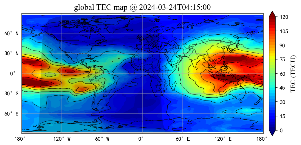
    ax.set_title(f'global TEC map @ {time_str}', fontsize=14, fontname='times new roman')
    
    ax.set_global()
    
    if output_path:
        plt.savefig(output_path, dpi=200, bbox_inches='tight')
        print(f"等高线图已保存: {output_path}")
    
    plt.show()
    ds.close()
if __name__ == "__main__":
    # 直接指定时间
    nc_file = r".\UPC_GIM_TEC_2024.nc"
    target_time = datetime(2024, 3, 24, 4, 15, 0)
    time_str = target_time.strftime('%Y%m%dT%H%M%S')
    # 检查文件是否存在
    if not os.path.exists(nc_file):
        print(f"文件 {nc_file} 不存在！")
    else:
        # 绘制TEC地图
        plot_tec_with_contour(
            nc_file_path=nc_file,
            target_time=target_time,
            output_path=f"global_tec_{time_str}.png"
        )

        print("\n程序执行完成！")

最终效果如下：

注意事项

依赖库 ：确保已安装 cartopy和 matplotlib。
日期处理 ：datetime对象应使用 UTC 时间，或自行处理时区转换。
地图投影 ：Nightshade会自动适配地图的投影方式，但某些极端投影（如极地投影）可能需要调整参数。