Day 1 编程实战：机器学习基础与评估指标

Day 1 编程实战：机器学习基础与评估指标

实战目标

1. 理解过拟合/欠拟合的概念
2. 掌握训练/验证/测试集划分
3. 熟练使用回归和分类评估指标
4. 用模拟数据完成完整ML流程

1. 导入必要的库

import numpy as np
import pandas as pd
import matplotlib.pyplot as plt
import seaborn as sns
from sklearn.datasets import make_regression, make_classification
from sklearn.model_selection import train_test_split, learning_curve
from sklearn.linear_model import LinearRegression, LogisticRegression
from sklearn.tree import DecisionTreeRegressor
from sklearn.metrics import (
    mean_squared_error, mean_absolute_error, r2_score,
    accuracy_score, precision_score, recall_score, f1_score,
    confusion_matrix, roc_auc_score, roc_curve, classification_report
)

# 启用LaTeX渲染（如果系统安装了LaTeX）
plt.rcParams['text.usetex'] = False  # 设为False避免LaTeX依赖

# 设置中文显示和美化
plt.rcParams['font.sans-serif'] = ['SimHei', 'Microsoft YaHei', 'DejaVu Sans']  # 用于中文显示
plt.rcParams['axes.unicode_minus'] = False  # 解决负号显示问题
# 在设置 seaborn 样式时直接传入字体配置
sns.set_style("whitegrid", {
    "font.sans-serif": ["SimHei", "Microsoft YaHei", "DejaVu Sans"],
    "axes.unicode_minus": False
})

2. 第一部分：回归任务 - 理解过拟合

2.1 生成非线性数据

# 生成非线性数据来演示过拟合
np.random.seed(42)
X = np.sort(5 * np.random.rand(80, 1), axis=0)
y = np.sin(X).ravel() + np.random.normal(0, 0.1, X.shape[0])

# 划分训练集和测试集
X_train, X_test, y_train, y_test = train_test_split(X, y, test_size=0.3, random_state=42)

# 可视化数据
plt.figure(figsize=(10, 6))
plt.scatter(X_train, y_train, color='blue', label='训练集', alpha=0.6)
plt.scatter(X_test, y_test, color='red', label='测试集', alpha=0.6)
plt.xlabel('特征 X')
plt.ylabel('目标值 y')
plt.title('生成的回归数据（非线性 + 噪声）')
plt.legend()
plt.show()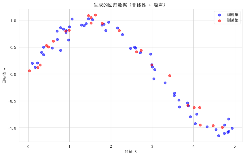

2.2 对比不同复杂度的模型

# 创建不同深度的决策树
depths = [1, 5, 20]  # 欠拟合、良好、过拟合
X_plot = np.linspace(0, 5, 500).reshape(-1, 1)

fig, axes = plt.subplots(1, 3, figsize=(15, 4))

for idx, depth in enumerate(depths):
    # 训练模型
    tree = DecisionTreeRegressor(max_depth=depth, random_state=42)
    tree.fit(X_train, y_train)
    
    # 预测
    y_train_pred = tree.predict(X_train)
    y_test_pred = tree.predict(X_test)
    y_plot_pred = tree.predict(X_plot)
    
    # 计算误差
    train_mse = mean_squared_error(y_train, y_train_pred)
    test_mse = mean_squared_error(y_test, y_test_pred)
    
    # 绘图
    axes[idx].scatter(X_train, y_train, color='blue', alpha=0.5, s=20, label='训练集')
    axes[idx].scatter(X_test, y_test, color='red', alpha=0.5, s=20, label='测试集')
    axes[idx].plot(X_plot, y_plot_pred, color='green', linewidth=2, label='模型预测')
    axes[idx].set_title(f'max_depth={depth}\n训练MSE={train_mse:.3f}, 测试MSE={test_mse:.3f}')
    axes[idx].set_xlabel('X')
    axes[idx].set_ylabel('y')
    axes[idx].legend()
    
    # 判断拟合状态
    if depth == 1:
        axes[idx].set_xlabel('欠拟合（Underfitting）')
    elif depth == 5:
        axes[idx].set_xlabel('良好拟合（Good Fit）')
    else:
        axes[idx].set_xlabel('过拟合（Overfitting）')

plt.tight_layout()
plt.show()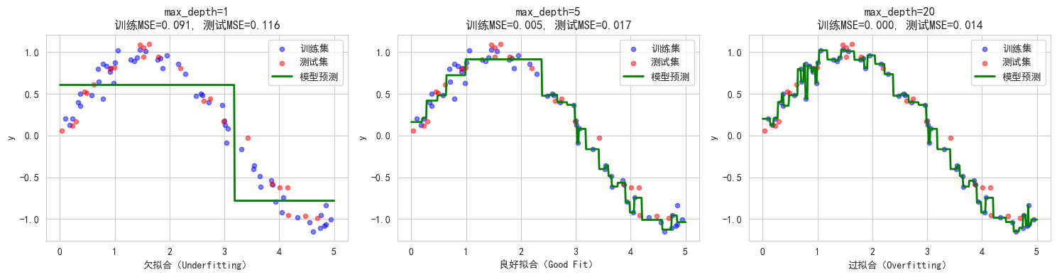

观察结论：

• max_depth=1：欠拟合，训练和测试误差都很高
• max_depth=5：良好拟合，训练和测试误差都较低
• max_depth=20：过拟合，训练误差极低但测试误差高

2.3 学习曲线 - 诊断过拟合

下面的代码定义了一个 学习曲线 的函数，这是一个非常重要的机器学习诊断工具。

def plot_learning_curve(estimator, X, y, title):
    """
    绘制学习曲线

    Parameters
        ----------
        estimator :
            机器学习模型对象（如回归树、线性回归等）
        X:
            特征矩阵
        y:
            目标变量
        title:
            图表标题
    """
    train_sizes, train_scores, test_scores = learning_curve(
        estimator, X, y, cv=5, n_jobs=-1,
        train_sizes=np.linspace(0.1, 1.0, 10),
        scoring='neg_mean_squared_error'
    )
    
    train_scores_mean = -np.mean(train_scores, axis=1)
    test_scores_mean = -np.mean(test_scores, axis=1)
    
    plt.figure(figsize=(8, 5))
    plt.plot(train_sizes, train_scores_mean, 'o-', label='训练误差', color='blue')
    plt.plot(train_sizes, test_scores_mean, 'o-', label='验证误差', color='red')
    plt.xlabel('训练样本数')
    plt.ylabel('MSE')
    plt.title(title)
    plt.legend()
    plt.grid(True)
    plt.show()

# 绘制过拟合模型的学习曲线
overfit_tree = DecisionTreeRegressor(max_depth=20, random_state=42)
plot_learning_curve(overfit_tree, X, y, '过拟合模型的学习曲线')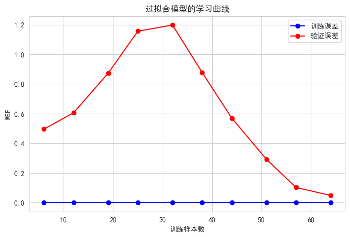

学习曲线解读：

• 训练误差很低，验证误差很高 → 过拟合
• 随着样本增加，验证误差下降 → 增加数据可缓解过拟合

learning_curve(): sklearn 函数，用于生成学习曲线

• cv=5: 使用5折交叉验证
• n_jobs=-1: 使用所有CPU核心加速计算
• train_sizes=np.linspace(0.1, 1.0, 10): 训练集大小比例从10%到100%，分成10个点
• scoring='neg_mean_squared_error': 使用负均方误差作为评估指标
• 返回值：
  • train_sizes: 训练集大小的比例数组
  • train_scores: 不同训练集大小下的训练得分（多折交叉验证的结果）
  • test_scores: 不同训练集大小下的验证得分

3. 第二部分：回归评估指标详解

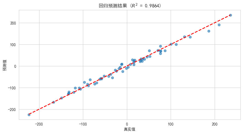
3.1 生成回归数据并计算指标

# 生成回归数据
X_reg, y_reg = make_regression(n_samples=200, n_features=1, noise=10, random_state=42)
X_train_r, X_test_r, y_train_r, y_test_r = train_test_split(X_reg, y_reg,
                                                            test_size=0.3,
                                                            random_state=42)

# 训练线性回归模型
lr = LinearRegression()
lr.fit(X_train_r, y_train_r)
y_pred_r = lr.predict(X_test_r)

# 计算各项指标
mse = mean_squared_error(y_test_r, y_pred_r)
mae = mean_absolute_error(y_test_r, y_pred_r)
r2 = r2_score(y_test_r, y_pred_r)

print("="*50)
print("回归评估指标结果")
print("="*50)
print(f"MSE (均方误差): {mse:.2f}")
print(f"MAE (平均绝对误差): {mae:.2f}")
print(f"R² (决定系数): {r2:.4f}")
print("="*50)

# 可视化预测结果
plt.figure(figsize=(10, 5))
plt.scatter(y_test_r, y_pred_r, alpha=0.6)
plt.plot([y_test_r.min(), y_test_r.max()], [y_test_r.min(), y_test_r.max()], 'r--', lw=2)
plt.xlabel('真实值')
plt.ylabel('预测值')
# plt.title(f'回归预测结果 (R² = {r2:.4f})')
plt.title(rf'回归预测结果 ($R^2$ = {r2:.4f})')  # 使用LaTeX格式
plt.grid(True)
plt.show()

==================================================
回归评估指标结果
==================================================
MSE (均方误差): 116.25
MAE (平均绝对误差): 8.42
R² (决定系数): 0.9864
==================================================

4. 第三部分：分类评估指标详解

4.1 生成不平衡分类数据

# 生成不平衡的二分类数据
X_clf, y_clf = make_classification(
    n_samples=1000, n_features=2, n_redundant=0, n_clusters_per_class=1,
    weights=[0.9, 0.1],  # 90%类别0，10%类别1
    flip_y=0.05, random_state=42
)

# 划分数据集
X_train_c, X_test_c, y_train_c, y_test_c = train_test_split(
    X_clf, y_clf, test_size=0.3, random_state=42, stratify=y_clf
)

# 训练逻辑回归模型
lr_clf = LogisticRegression(random_state=42)
lr_clf.fit(X_train_c, y_train_c)
y_pred_c = lr_clf.predict(X_test_c)
y_pred_proba_c = lr_clf.predict_proba(X_test_c)[:, 1]

# 计算各项指标
accuracy = accuracy_score(y_test_c, y_pred_c)
precision = precision_score(y_test_c, y_pred_c)
recall = recall_score(y_test_c, y_pred_c)
f1 = f1_score(y_test_c, y_pred_c)
auc = roc_auc_score(y_test_c, y_pred_proba_c)

print("="*50)
print("分类评估指标结果")
print("="*50)
print(f"准确率 (Accuracy): {accuracy:.4f}")
print(f"精确率 (Precision): {precision:.4f}")
print(f"召回率 (Recall): {recall:.4f}")
print(f"F1分数: {f1:.4f}")
print(f"AUC: {auc:.4f}")
print("="*50)

==================================================
分类评估指标结果
==================================================
准确率 (Accuracy): 0.9600
精确率 (Precision): 1.0000
召回率 (Recall): 0.6571
F1分数: 0.7931
AUC: 0.8790
==================================================

y_pred_proba_c = lr_clf.predict_proba(X_test_c)[:, 1]

predict_proba() 方法

• 作用：返回每个类别的预测概率
• 返回值：二维数组，形状为 (n_samples, n_classes)
  • 每行是一个样本的各类别概率
  • 每行的概率和为1

切片 [:, 1] ：

• 所有行，第1列（索引从0开始）
• 二分类：0列是类别0的概率，1列是列别1（正类）的概率

4.2 混淆矩阵可视化

# 混淆矩阵
cm = confusion_matrix(y_test_c, y_pred_c)

plt.figure(figsize=(4, 3))
sns.heatmap(cm, annot=True, fmt='d', cmap='Blues', 
            xticklabels=['预测下跌', '预测上涨'],
            yticklabels=['实际下跌', '实际上涨'])
plt.title('混淆矩阵')
plt.ylabel('真实标签')
plt.xlabel('预测标签')
plt.show()

# 打印详细分类报告
print("\n分类报告（Classification Report）:")
print(classification_report(y_test_c, y_pred_c, target_names=['下跌', '上涨']))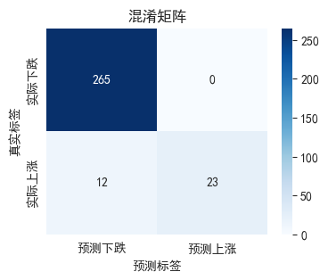

​

分类报告（Classification Report）:

precision recall f1-score support

          下跌       0.96      1.00      0.98       265
          上涨       1.00      0.66      0.79        35

    accuracy                           0.96       300
   macro avg       0.98      0.83      0.89       300
weighted avg       0.96      0.96      0.96       300

​

解读混淆矩阵：

• TP: 正确预测上涨的数量
• TN: 正确预测下跌的数量
• FP: 误报（预测涨实际跌）
• FN: 漏报（预测跌实际涨）

4.3 ROC曲线与AUC

# 计算ROC曲线
fpr, tpr, thresholds = roc_curve(y_test_c, y_pred_proba_c)

plt.figure(figsize=(4, 3))
plt.plot(fpr, tpr, linewidth=2, label=f'ROC曲线 (AUC = {auc:.4f})')
plt.plot([0, 1], [0, 1], 'k--', linewidth=1, label='随机分类器 (AUC=0.5)')
plt.fill_between(fpr, tpr, alpha=0.2)
plt.xlabel('假阳性率 (False Positive Rate)')
plt.ylabel('真阳性率 (True Positive Rate)')
plt.title('ROC曲线')
plt.legend(loc='lower right')
plt.grid(True)
plt.show()

# 不同阈值下的性能
print("\n不同阈值下的性能:")
for threshold in [0.3, 0.5, 0.7]:
    y_pred_thresh = (y_pred_proba_c >= threshold).astype(int)
    precision_thresh = precision_score(y_test_c, y_pred_thresh)
    recall_thresh = recall_score(y_test_c, y_pred_thresh)
    print(f"阈值={threshold:.1f}: 精确率={precision_thresh:.3f}, 召回率={recall_thresh:.3f}")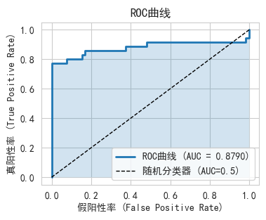

​

不同阈值下的性能:

阈值=0.3: 精确率=1.000, 召回率=0.714

阈值=0.5: 精确率=1.000, 召回率=0.657

阈值=0.7: 精确率=1.000, 召回率=0.600

ROC曲线解读：

• 曲线越靠近左上角，模型越好
• AUC=0.5表示随机猜测
• AUC=1.0表示完美分类器

5. 第四部分：数据集划分实战

5.1 模拟时间序列数据（量化场景）

# 生成模拟股票数据
np.random.seed(42)
dates = pd.date_range('2020-01-01', periods=500, freq='D')
returns = np.random.randn(500) * 0.02  # 模拟日收益率
price = 100 + np.cumsum(returns) * 100

df = pd.DataFrame({
    'date': dates,
    'price': price,
    'return': returns
})
df['target'] = (df['return'].shift(-1) > 0).astype(int)  # 次日是否上涨
df = df.dropna()

print("数据形状:", df.shape)
df.head()

数据形状: (500, 4)

| | date | price | return | target |
| 0 | 2020-01-01 | 100.993428 | 0.009934 | 0 |
| 1 | 2020-01-02 | 100.716900 | -0.002765 | 1 |
| 2 | 2020-01-03 | 102.012277 | 0.012954 | 1 |
| 3 | 2020-01-04 | 105.058336 | 0.030461 | 0 |

4	2020-01-05	104.590030	-0.004683	0

# 正确的划分方式：按时间顺序
split_date = '2020-12-18'
train_df = df[df['date'] < split_date]
test_df = df[df['date'] >= split_date]

print(f"训练集大小: {len(train_df)} ({split_date}之前)")
print(f"测试集大小: {len(test_df)} ({split_date}之后)")

# 特征和标签
feature_cols = ['return', 'price']
X_train_ts = train_df[feature_cols]
y_train_ts = train_df['target']
X_test_ts = test_df[feature_cols]
y_test_ts = test_df['target']

# 训练和评估
model = LogisticRegression()
model.fit(X_train_ts, y_train_ts)
y_pred_ts = model.predict(X_test_ts)
print(f"\n测试集准确率: {accuracy_score(y_test_ts, y_pred_ts):.4f}")

训练集大小: 352 (2020-12-18之前)
测试集大小: 148 (2020-12-18之后)

测试集准确率: 0.5203

5.2 错误做法对比：随机划分（会导致前视偏差）

# 错误做法：随机划分
X_train_wrong, X_test_wrong, y_train_wrong, y_test_wrong = train_test_split(
    df[feature_cols], df['target'], test_size=0.3, random_state=42, shuffle=True
)

# 这会导致模型使用未来信息训练，测试集可能在时间上早于训练集
print("错误做法警告：随机划分会破坏时间顺序，导致前视偏差！")
print("训练集最后日期可能晚于测试集最早日期")

错误做法警告：随机划分会破坏时间顺序，导致前视偏差！
训练集最后日期可能晚于测试集最早日期

6. 第五部分：综合练习

6.1 练习1：评估指标计算（手动实现）

def calculate_metrics_manual(y_true, y_pred, y_pred_proba=None):
    """手动实现评估指标"""
    # 混淆矩阵
    tp = np.sum((y_true == 1) & (y_pred == 1))
    tn = np.sum((y_true == 0) & (y_pred == 0))
    fp = np.sum((y_true == 0) & (y_pred == 1))
    fn = np.sum((y_true == 1) & (y_pred == 0))
    
    # 基础指标
    accuracy = (tp + tn) / (tp + tn + fp + fn)
    precision = tp / (tp + fp) if (tp + fp) > 0 else 0
    recall = tp / (tp + fn) if (tp + fn) > 0 else 0
    f1 = 2 * (precision * recall) / (precision + recall) if (precision + recall) > 0 else 0
    
    return {
        '混淆矩阵': {'TP': tp, 'TN': tn, 'FP': fp, 'FN': fn},
        '准确率': accuracy,
        '精确率': precision,
        '召回率': recall,
        'F1分数': f1
    }

# 测试手动实现
from sklearn.metrics import precision_score, recall_score, f1_score

y_true_test = np.array([1, 0, 1, 1, 0, 1, 0, 0, 1, 0])
y_pred_test = np.array([1, 0, 1, 0, 0, 1, 0, 1, 1, 0])

manual_results = calculate_metrics_manual(y_true_test, y_pred_test)
sklearn_precision = precision_score(y_true_test, y_pred_test)
sklearn_recall = recall_score(y_true_test, y_pred_test)
sklearn_f1 = f1_score(y_true_test, y_pred_test)

print("手动实现结果:")
print(f"精确率: {manual_results['精确率']:.4f}")
print(f"召回率: {manual_results['召回率']:.4f}")
print(f"F1分数: {manual_results['F1分数']:.4f}")
print("\nsklearn结果:")
print(f"精确率: {sklearn_precision:.4f}")
print(f"召回率: {sklearn_recall:.4f}")
print(f"F1分数: {sklearn_f1:.4f}")

手动实现结果:
精确率: 0.8000
召回率: 0.8000
F1分数: 0.8000

sklearn结果:
精确率: 0.8000
召回率: 0.8000
F1分数: 0.8000

6.2 练习2：过拟合实验

# 生成非线性数据来演示过拟合
np.random.seed(42)
X = np.sort(5 * np.random.rand(1000, 1), axis=0)
y = np.sin(X).ravel() + np.random.normal(0, 0.1, X.shape[0])

# 在不同训练集大小下观察过拟合
train_sizes = [50, 100, 200, 400, 800]
test_errors = []
train_errors = []

for size in train_sizes:
    # 取前size个样本
    X_train_sub = X[:size]
    y_train_sub = y[:size]
    
    # 训练过拟合模型
    tree = DecisionTreeRegressor(max_depth=20, random_state=42)
    tree.fit(X_train_sub, y_train_sub)
    
    # 计算误差
    train_mse = mean_squared_error(y[:size], tree.predict(X[:size]))
    test_mse = mean_squared_error(y[size:], tree.predict(X[size:]))
    
    train_errors.append(train_mse)
    test_errors.append(test_mse)

plt.figure(figsize=(5, 3))
plt.plot(train_sizes, train_errors, 'o-', label='训练误差', color='blue')
plt.plot(train_sizes, test_errors, 'o-', label='测试误差', color='red')
plt.xlabel('训练样本数')
plt.ylabel('MSE')
plt.title('训练集大小对过拟合的影响')
plt.legend()
plt.grid(True)
plt.show()

print("\n结论：随着训练样本增加，过拟合程度降低（测试误差下降）")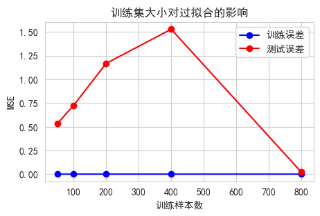

结论：随着训练样本增加，过拟合程度降低（测试误差下降）

7. 第六部分：今日总结

今日学习要点总结

核心概念：

1. 监督学习、无监督学习、强化学习的区别
2. 过拟合：训练好但测试差；欠拟合：训练测试都差
3. 数据划分：训练集→验证集→测试集

回归指标：

• MSE：对异常值敏感
• MAE：更鲁棒
• R²：解释方差的比例

分类指标：

• 准确率：类别平衡时好用
• 精确率：减少误报
• 召回率：减少漏报
• F1：精确率和召回率的平衡
• AUC：不受类别不平衡影响

量化注意事项：

• 必须按时间顺序划分数据
• 使用时间序列交叉验证
• 警惕前视偏差

扩展阅读与作业

作业：

1. 修改过拟合实验中的max_depth参数，找到最优值
2. 在不平衡分类数据上，对比使用不同评估指标的结果差异
3. 查找资料：为什么金融数据不能使用普通K折交叉验证？