基于 PyTorch 的 Fashion-MNIST CNN 分类模型

Fashion-MNIST Classification with CNN in PyTorch

Fashion MNIST dataset：https://www.kaggle.com/datasets/zalando-research/fashionmnist.

本文实现了一个基于卷积神经网络（CNN）的 Fashion-MNIST 图像分类模型，完整覆盖了从数据预处理、模型构建、训练优化到推理预测的全过程。

This project implements a Convolutional Neural Network (CNN) for Fashion-MNIST image classification, covering the full pipeline from data preprocessing and model design to training and inference.

核心目标是构建一个结构清晰、可解释性强的经典 CNN（LeNet 风格），并重点展示深度学习中的关键算法技术。

The goal is to build a clean and interpretable LeNet-style CNN while highlighting key algorithmic techniques in deep learning.

1. 数据加载与预处理

1. Data Loading and Preprocessing

1.1 使用Pandas读取CSV数据

1.1 Reading CSV Data with Pandas

python 复制代码

train_data = pd.read_csv("../data/fashion-mnist_train.csv")
test_data = pd.read_csv("../data/fashion-mnist_train.csv")

x_train = train_data.iloc[:, :-1].values  # All columns except first (pixel values)
y_train = train_data.iloc[:, 0].values    # First column (labels)
x_test = train_data.iloc[:, 1:].values    # Pixel values for test
y_test = train_data.iloc[:, 0].values     # Labels for test

第一列包含类别标签（0-9），其余784列代表展开的28×28像素值。我们使用iloc分离特征和标签。

The first column contains class labels (0-9), while the remaining 784 columns represent flattened 28×28 pixel values. We use iloc to separate features and labels.

1.2 转换为PyTorch张量并重塑形状

1.2 Converting to PyTorch Tensors and Reshaping

python 复制代码

x_train = torch.from_numpy(x_train).float().reshape(-1, 1, 28, 28)
x_test = torch.from_numpy(x_test).float().reshape(-1, 1, 28, 28)
y_train = torch.tensor(y_train)
y_test = torch.tensor(y_test)
print(x_train.shape, y_train.shape)  # torch.Size([60000, 1, 28, 28]) torch.Size([60000])

重塑操作将数据从(N, 784)转换为(N, 1, 28, 28)，其中1表示Conv2d层所需的灰度通道维度

The reshape operation transforms data from (N, 784) to (N, 1, 28, 28), where 1 represents the grayscale channel dimension required by Conv2d layers.

1.3 构建数据集和数据加载器

1.3 Building Dataset and DataLoader

python 复制代码

train_dataset = TensorDataset(x_train, y_train)
test_dataset = TensorDataset(x_test, y_test)

batch_size = 256
train_loader = DataLoader(dataset=train_dataset, batch_size=batch_size, shuffle=True)
test_loader = DataLoader(dataset=test_dataset, batch_size=batch_size)

TensorDataset将张量包装成数据集，而DataLoader实现了训练数据的mini-batch迭代和随机打乱。

TensorDataset wraps tensors into a dataset, while DataLoader enables mini-batch iteration with random shuffling for training data.

2. 模型架构：LeNet风格卷积神经网络

2. Model Architecture: LeNet-Style CNN

2.1 序列模型定义

2.1 Sequential Model Definition

python 复制代码

model = nn.Sequential(
    # First convolutional layer: 1→6 channels, 5×5 kernel, padding=2 (keeps 28×28)
    # 第一卷积层：1→6通道，5×5卷积核，padding=2（保持28×28尺寸）
    nn.Conv2d(1, 6, kernel_size=5, padding=2),
    nn.Sigmoid(),
    nn.AvgPool2d(kernel_size=2, stride=2),  # 28×28 → 14×14
    
    # Second convolutional layer: 6→16 channels, 5×5 kernel
    # 第二卷积层：6→16通道，5×5卷积核
    nn.Conv2d(6, 16, kernel_size=5),
    nn.Sigmoid(),
    nn.AvgPool2d(kernel_size=2, stride=2),  # 14×14 → 7×7 (actually 10×10 → 5×5? Let's check)
    
    nn.Flatten(),  # Flatten: 16×5×5 = 400 → 1D vector / 展平：16×5×5 = 400 → 一维向量
    nn.Linear(400, 120),
    nn.Sigmoid(),
    nn.Linear(120, 84),
    nn.Sigmoid(),
    nn.Linear(84, 10),  # Output: 10 classes / 输出：10个类别
)

层	作用

|--------|---------------|
| Conv2d | 局部特征提取（卷积核扫描） |

|---------|-------|
| Sigmoid | 非线性映射 |

|---------|-----|
| AvgPool | 降采样 |

|--------|------|
| Linear | 分类决策 |

该架构遵循LeNet-5设计，包含两个Conv-Sigmoid-AvgPool模块，后接三个全连接层。最后一层输出10个时尚类别的logits。

This architecture follows LeNet-5 design with two Conv-Sigmoid-AvgPool blocks followed by three fully-connected layers. The final layer outputs logits for 10 fashion categories.

2.2 前向传播形状验证

2.2 Forward Shape Verification

python 复制代码

x = torch.randn(1, 1, 28, 28)
for layer in model:
    x = layer(x)
    print(f"{layer.__class__.__name__:<12} output shape: {x.shape}")

# Output / 输出:
# Conv2d       output shape: torch.Size([1, 6, 28, 28])
# Sigmoid      output shape: torch.Size([1, 6, 28, 28])
# AvgPool2d    output shape: torch.Size([1, 6, 14, 14])
# Conv2d       output shape: torch.Size([1, 16, 10, 10])
# Sigmoid      output shape: torch.Size([1, 16, 10, 10])
# AvgPool2d    output shape: torch.Size([1, 16, 5, 5])
# Flatten      output shape: torch.Size([1, 400])
# Linear       output shape: torch.Size([1, 120])
# Sigmoid      output shape: torch.Size([1, 120])
# Linear       output shape: torch.Size([1, 84])
# Sigmoid      output shape: torch.Size([1, 84])
# Linear       output shape: torch.Size([1, 10])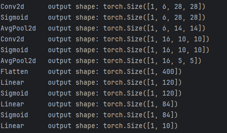

形状验证确保每一层的输出维度与下一层的预期输入匹配，防止运行时维度不匹配错误。

Shape verification ensures each layer's output dimensions match the next layer's expected input, preventing runtime dimension mismatch errors.

3. 用于稳定收敛的Xavier初始化

3. Xavier Initialization for Stable Convergence

python 复制代码

def init_weights(layer):
    if isinstance(layer, nn.Linear) or isinstance(layer, nn.Conv2d):
        nn.init.xavier_uniform_(layer.weight)

model.apply(init_weights)

Xavier均匀初始化将初始权重方差设为2/(fan_in + fan_out)，可防止Sigmoid激活网络中的梯度消失或爆炸问题。

Xavier uniform initialization sets initial weights with variance 2/(fan_in + fan_out), which prevents gradients from vanishing or exploding in Sigmoid-activated networks.

4. 训练设置：损失函数与优化器

4. Training Setup: Loss Function and Optimizer

python 复制代码

device = torch.device("cuda:0" if torch.cuda.is_available() else "cpu")
model.to(device)

lr = 0.9  # Learning rate / 学习率
epochs = 20

loss_func = nn.CrossEntropyLoss()  # Combines LogSoftmax + NLLLoss
optimizer = optim.SGD(model.parameters(), lr=lr)  # Stochastic Gradient Descent

CrossEntropyLoss是多分类的标准选择，它结合了softmax激活和负对数似然损失。可以添加带动量的SGD以加快收敛速度。

CrossEntropyLoss is the standard choice for multi-class classification, combining softmax activation and negative log-likelihood loss. SGD with momentum could be added for faster convergence.

5. 带实时监控的训练循环

5. Training Loop with Real-Time Monitoring

python 复制代码

for epoch in range(epochs):
    # Training phase / 训练阶段
    model.train()
    train_loss = 0
    train_acc_num = 0
    
    for i, (X, y) in enumerate(train_loader):
        X, target = X.to(device), y.to(device)
        
        # Forward pass / 前向传播
        output = model(X)
        loss = loss_func(output, target)
        
        # Backward pass / 反向传播
        loss.backward()
        optimizer.step()
        optimizer.zero_grad()
        
        # Accumulate metrics / 累计指标
        train_loss += loss.item() * X.shape[0]
        y_pred = output.argmax(dim=1)
        train_acc_num += y_pred.eq(target).sum().item()
    
    # Calculate epoch metrics / 计算本轮指标
    this_train_loss = train_loss / len(train_dataset)
    this_train_acc = train_acc_num / len(train_dataset)
    
    # Validation phase / 验证阶段
    model.eval()
    val_loss = 0
    val_acc_num = 0
    
    with torch.no_grad():  # Disable gradient computation / 禁用梯度计算
        for X, target in test_loader:
            X, target = X.to(device), target.to(device)
            output = model(X)
            loss = loss_func(output, target)
            val_loss += loss.item() * X.shape[0]
            y_pred = output.argmax(dim=1)
            val_acc_num += y_pred.eq(target).sum().item()
    
    this_val_loss = val_loss / len(test_dataset)
    this_val_acc = val_acc_num / len(test_dataset)
    
    print(f"Epoch:{epoch+1}, train loss:{this_train_loss:.4f}, train acc:{this_train_acc:.4f}, "
          f"val loss:{this_val_loss:.4f}, val acc:{this_val_acc:.4f}")

训练循环在训练阶段和验证阶段之间交替。model.train()启用dropout/批归一化行为，而model.eval()禁用它们。torch.no_grad()在验证期间减少内存使用。

The training loop alternates between training and validation phases. model.train() enables dropout/batch norm behaviors, while model.eval() disables them. torch.no_grad() reduces memory usage during validation.

6. 预测与可视化

6. Prediction and Visualization

python 复制代码

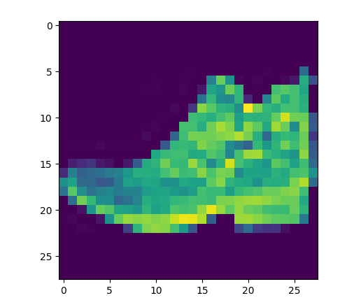
# Select a single test sample / 选择单个测试样本
x_new = x_test[666]
plt.imshow(x_new[0], cmap='gray')
plt.title(f"True Label: {y_test[666]}")
plt.show()

# Model prediction / 模型预测
output = model(x_new.unsqueeze(0).to(device))  # Add batch dimension / 添加批次维度
y_pred = output.argmax(dim=1)
print(f"Predicted Label: {y_pred.item()}")

unsqueeze(0)操作添加一个批次维度，将形状从(1,28,28)转换为(1,1,28,28)以匹配模型期望的输入格式。

The unsqueeze(0) operation adds a batch dimension, converting shape from (1,28,28) to (1,1,28,28) to match the model's expected input format.

7.完整代码

python 复制代码

"""
Fashion-MNIST 图像分类模型（PyTorch CNN）
1. 数据处理：使用 pandas 读取 CSV 格式 Fashion-MNIST 数据集，并转换为 PyTorch Tensor，调整为 (N, 1, 28, 28) 的 CNN 输入格式。
2. 数据集构建：使用 TensorDataset + DataLoader 实现 mini-batch 训练与随机打乱。
3. 模型结构：采用经典 LeNet 风格 CNN，包括：
   - 两层卷积层（Conv2d）
   - Sigmoid 激活函数
   - 平均池化层（AvgPool2d）
   - 全连接层（Linear）
   - Flatten 展平操作
   输出为 10 类分类结果。
4. 参数初始化：对 Conv2d 和 Linear 层使用 Xavier初始化，提高收敛稳定性。
5. 损失函数：使用 CrossEntropyLoss 作为多分类标准损失函数。
6. 优化方法：使用 SGD 随机梯度下降优化器进行参数更新。
7. 训练策略：采用 mini-batch 训练方式，计算训练/验证集 loss 与 accuracy，并实时监控训练过程。
8. 评估方式：使用 argmax 进行类别预测，并计算分类准确率。
9. 推理阶段：对单张测试图像进行可视化，并使用模型进行类别预测。
"""

import torch
import pandas as pd
import torch.nn as nn
import matplotlib.pyplot as plt
import torch.optim as optim
from torch.utils.data import TensorDataset, DataLoader

train_data = pd.read_csv("../data/fashion-mnist_train.csv")
test_data = pd.read_csv("../data/fashion-mnist_train.csv")

x_train= train_data.iloc[:, :-1].values
y_train= train_data.iloc[:, 0].values
x_test= train_data.iloc[:, 1:].values
y_test= train_data.iloc[:, 0].values

#转换为tensor
x_train= torch.from_numpy(x_train).float().reshape(-1,1,28,28)
x_test= torch.from_numpy(x_test).float().reshape(-1,1,28,28)
y_train=torch.tensor(y_train)
y_test=torch.tensor(y_test)
print(x_train.shape, y_train.shape)
print(x_test.shape, y_test.shape)

# plt.imshow(x_train[0,0],cmap='gray')
# plt.show()
# print(y_train[0])#真实标签

#构建数据集
train_dataset = TensorDataset(x_train, y_train)
test_dataset = TensorDataset(x_test, y_test)

# 搭建模型
model = nn.Sequential(
    nn.Conv2d(1, 6, kernel_size=5, padding=2),
    nn.Sigmoid(),
nn.AvgPool2d(kernel_size=2, stride=2),

    nn.Conv2d(6, 16, kernel_size=5),
    nn.Sigmoid(),
nn.AvgPool2d(kernel_size=2, stride=2),

    nn.Flatten(),  # 拉平
    nn.Linear(400, 120),
nn.Sigmoid(),

    nn.Linear(120, 84),
nn.Sigmoid(),


    nn.Linear(84, 10),
)
#测试每层前向传播的形状
x=torch.randn(1, 1, 28, 28)
for layer in model:
    x=layer(x)
    print(f"{layer.__class__.__name__:<12}output shape: {x.shape}")

#参数初始化
def init_weights(layers):
    if isinstance(layer, nn.Linear)or isinstance(layer, nn.Conv2d):
        nn.init.xavier_uniform_(layer.weight)
model.apply(init_weights)

#定义设备
device=torch.device("cuda:0" if torch.cuda.is_available() else "cpu")
model.to(device)

#设置超参数
lr=0.9
batch_size=256
epochs=20

#创建数据加载器
train_loader = DataLoader(dataset=test_dataset, batch_size=batch_size, shuffle=True)
test_loader=DataLoader(dataset=test_dataset, batch_size=batch_size)

#损失函数和优化器
loss_func=nn.CrossEntropyLoss()
optimizer=optim.SGD(model.parameters(), lr=lr)#AdamW

#模型训练
for epoch in range(epochs):
    #训练过程
    model.train()
    train_loss = 0
    train_acc_num = 0
    #按小批次遍历训练集
    for i,(X,y) in enumerate(train_loader):
        X,target=X.to(device),y.to(device)
        #前向传播
        output=model(X)
        #计算损失
        loss=loss_func(output,target)
        #反向传播
        loss.backward()
        #更新参数
        optimizer.step()
        #梯度清零
        optimizer.zero_grad()
        #累加训练损失
        train_loss += loss.item()*X.shape[0]
        # 累加预测正确的数量
        y_pred=output.argmax(dim=1)
        train_acc_num+=y_pred.eq(target).sum().item()
        #进度条
        print(f"\rEpoch:{epoch+1:0>3} [{'='* int((i+1)/len(train_loader)*50):<50}]",end=" ")
    #本轮训练完毕，计算平均顺势和准确率
    this_train_loss = train_loss/len(train_dataset)
    this_train_acc = train_acc_num/len(train_dataset)

    #验证
    model.eval()
    val_loss = 0
    val_acc_num = 0
    with torch.no_grad():
        for X,target in test_loader:
            X,target=X.to(device),target.to(device)
            #前向传播
            output=model(X)
            #计算损失
            loss=loss_func(output,target)
            #累加验证损失
            val_loss += loss.item()*X.shape[0]
            #累加预测正确的数量
            y_pred=output.argmax(dim=1)
            val_acc_num+=y_pred.eq(target).sum().item()
    this_train_loss = val_loss/len(test_dataset)
    this_train_acc = val_acc_num/len(test_dataset)

    print(f"Epoch:{epoch+1},train loss:{this_train_loss:.4f},train acc:{this_train_acc:.4f},"
          f"val loss:{this_train_loss:.4f},val acc:{this_train_acc:.4f}")

#5测试(预测）
x_new=x_test[666]
plt.imshow(x_new[0])
plt.show()
print(y_test[666])#正确分类标签

#用模型预测分类
output=model(x_new.unsqueeze(0).to(device))
y_pred=output.argmax(dim=1)
print(y_pred)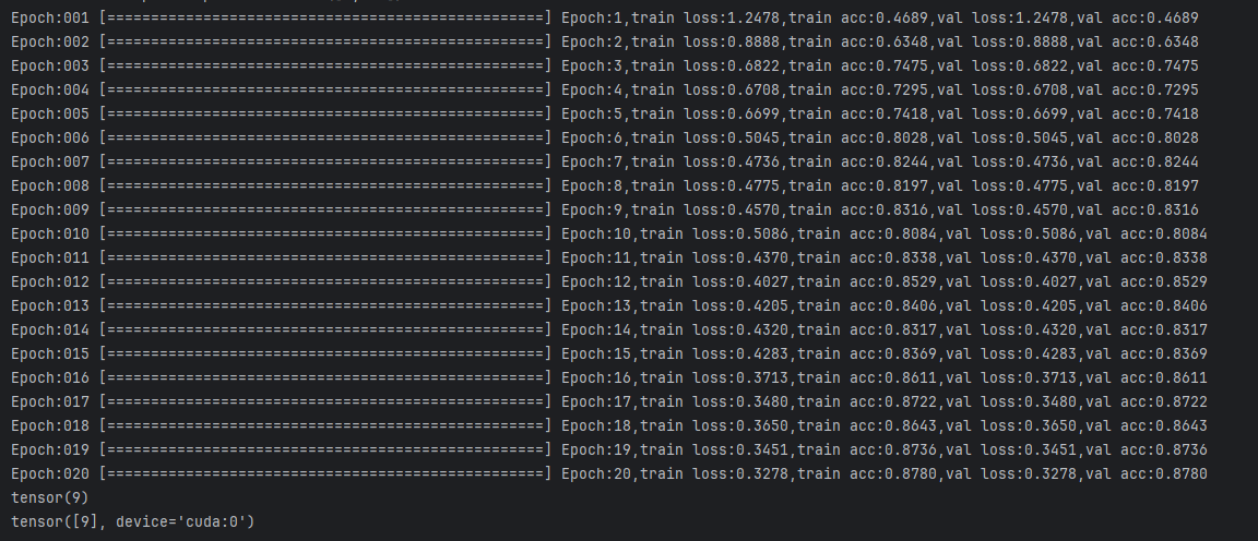

预测结果：tensor(9)

标签：tensor([9])