Q/K/V 三件套：把 Bahdanau 抽象成一个公式

如果你只读本系列的一篇，这一篇的优先级最高。

Q、K、V 这三个字母，是从 Bahdanau 的 additive attention 抽象出来的「三件套」。一旦把这三件套立起来，Transformer、cross-attention、multi-head、causal mask、KV cache、FlashAttention------后面所有 attention 相关的概念，都只是「三件套的不同排列组合」。

这一篇会用最长的篇幅、最具体的数字，把 Q/K/V 讲透。读完之后你应该能做到：

看到 <math xmlns="http://www.w3.org/1998/Math/MathML"> s o f t m a x ( Q K ⊤ / d k ) V softmax(QK^\top/\sqrt{d_k})V </math>softmax(QK⊤/dk )V 这一行，立刻在脑子里把每一项的语义、形状、来历说清楚；
理解为什么 K 和 V 要分开（即使它们经常用同一份输入投影出来）；
在草稿纸上手算一个三 token、d_k=2 的最小例子，且每一步的形状都对得上。

先把这条主公式贴出来，然后我们一节一节地拆它：
<math xmlns="http://www.w3.org/1998/Math/MathML" display="block"> Attention ( Q , K , V ) = softmax ( Q K ⊤ d k ) V \text{Attention}(Q, K, V) = \text{softmax}\left(\frac{QK^\top}{\sqrt{d_k}}\right) V </math>Attention(Q,K,V)=softmax(dk QK⊤)V

0、先看两张经典图

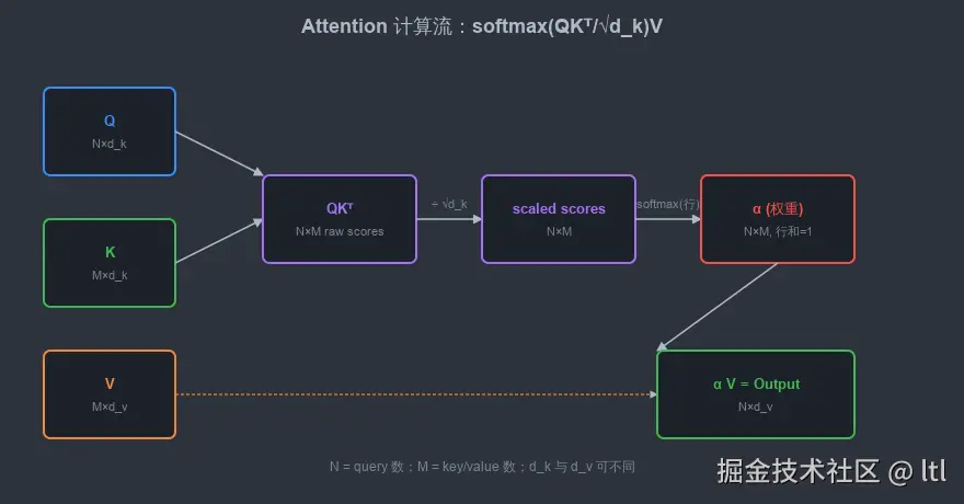
下面两张图可以先建立一个整体直觉，再继续读后面的逐项拆解：

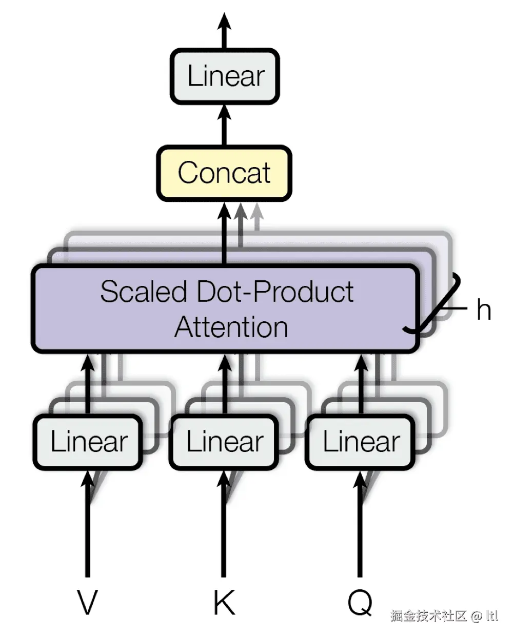
第一张是 Scaled Dot-Product Attention（展示 <math xmlns="http://www.w3.org/1998/Math/MathML"> Q K ⊤ / d k QK^\top / \sqrt{d_k} </math>QK⊤/dk 与 softmax 后再乘 <math xmlns="http://www.w3.org/1998/Math/MathML"> V V </math>V 的主流程）。

第二张是 Transformer 总体结构图（标出 encoder/decoder 内的 attention 模块位置）。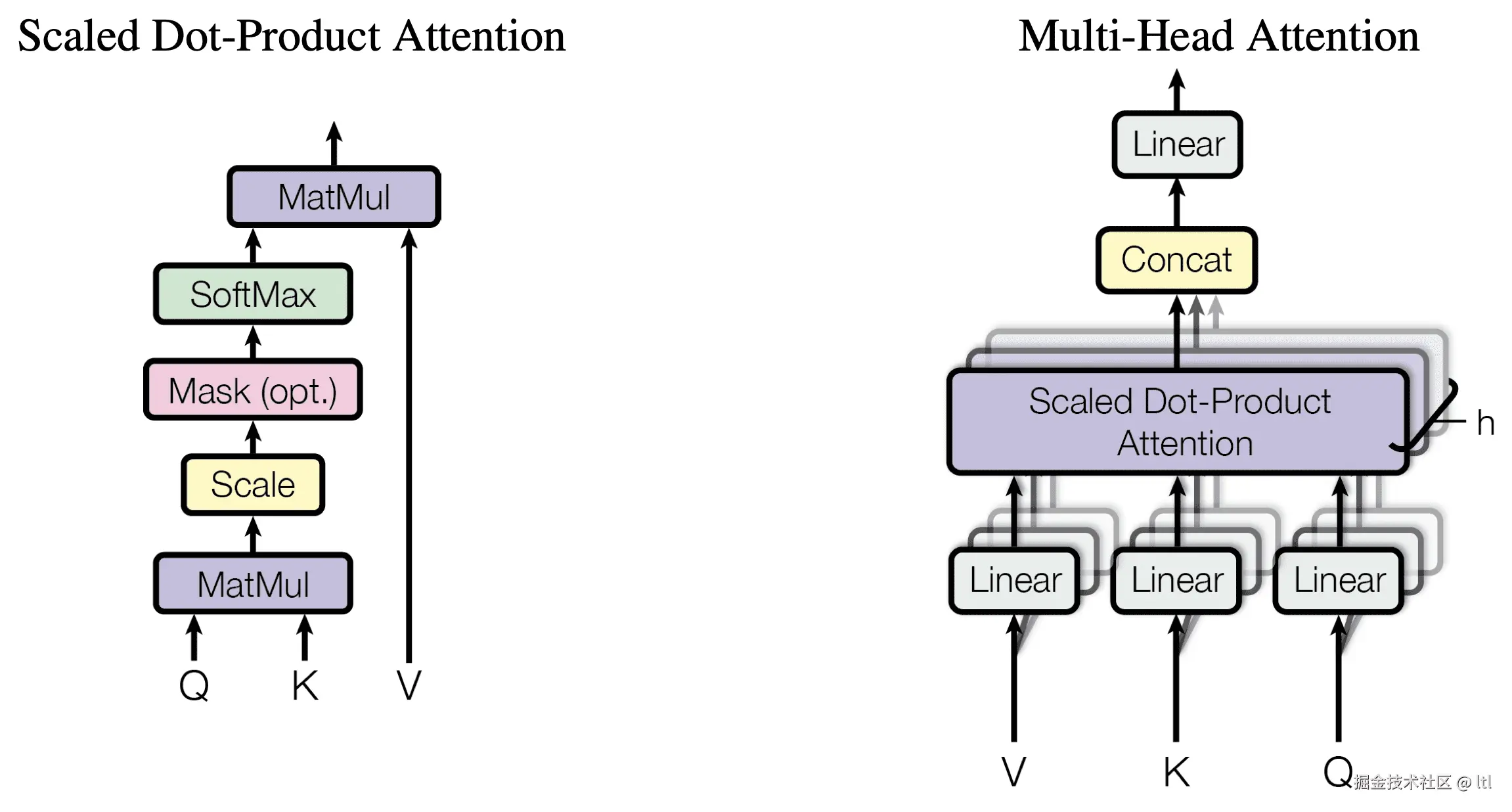

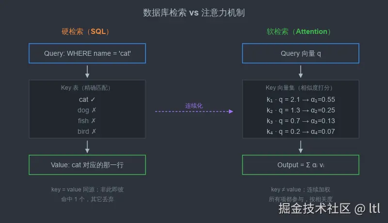
一、信息检索：从硬命中到软加权

1.1 一个数据库查询

先抛开神经网络，回到 SQL。

你有一张 animals 表，三列：id、name、description。

你跑一条查询：

sql 复制代码

SELECT description FROM animals WHERE name = 'cat';

数据库做了三件事：

第一，把你输入的 'cat' 当成 Query（查询条件）。

第二，遍历表里每一行的 name 字段，作为 Key，与 Query 比较是否相等。

第三，对命中的那一行，返回它的 description 字段------也就是 Value。

注意这里 Key 和 Value 来自同一张表的不同列：name 是「索引」，description 是「内容」。

它们刻意分开，就是为了让「索引」和「内容」可以独立设计------你用 name 找，但拿回的是 description。

1.2 硬检索的局限

SQL 的检索是「硬」的：

命中 = 1，没命中 = 0；
一次查询要么返回一行、要么返回零行（精确匹配）；
多个候选若都满足条件，结果是它们的并集，不是「按相关度加权」。

这套范式在结构化数据上完美无瑕，但对自然语言、图像、连续表示来说，不行。

name = 'cat' 这种相等判断，对「kitty」、「feline」、「the cat sat on the mat」都会失败。

我们需要一种相似度查询：「query 与 key 有多像？相似度越高，权重越大。」

而且「权重」最好是连续的、可微的------这样神经网络能反向传播。

1.3 软检索的形式化

把硬检索软化，结果就是 attention：

概念	硬检索	软检索（attention）
Query	一个值	一个向量 <math xmlns="http://www.w3.org/1998/Math/MathML"> q q </math>q
Key	字段（精确匹配）	一组向量 <math xmlns="http://www.w3.org/1998/Math/MathML"> { k 1 , ... , k M } \{k_1, \ldots, k_M\} </math>{k1,...,kM}
Value	命中行的另一个字段	一组向量 <math xmlns="http://www.w3.org/1998/Math/MathML"> { v 1 , ... , v M } \{v_1, \ldots, v_M\} </math>{v1,...,vM}
相似度	等号判断（ <math xmlns="http://www.w3.org/1998/Math/MathML"> 0 / 1 0/1 </math>0/1）	内积或 MLP 打分（实数）
选择	命中即返回	<math xmlns="http://www.w3.org/1998/Math/MathML"> softmax ⁡ \operatorname{softmax} </math>softmax 归一化为权重，所有候选都参与加权
输出	单条记录	<math xmlns="http://www.w3.org/1998/Math/MathML"> ∑ i α i v i \sum_i \alpha_i v_i </math>∑iαivi，所有 value 的加权和

如果把「软检索」正式写成公式，单个 query 的 attention 就是：
<math xmlns="http://www.w3.org/1998/Math/MathML" display="block"> s i = score ⁡ ( q , k i ) α i = exp ⁡ ( s i ) ∑ j = 1 M exp ⁡ ( s j ) o = ∑ i = 1 M α i v i \begin{aligned} s_i &= \operatorname{score}(q, k_i) \\ \alpha_i &= \frac{\exp(s_i)}{\sum_{j=1}^{M} \exp(s_j)} \\ o &= \sum_{i=1}^{M} \alpha_i v_i \end{aligned} </math>siαio=score(q,ki)=∑j=1Mexp(sj)exp(si)=i=1∑Mαivi

其中， <math xmlns="http://www.w3.org/1998/Math/MathML"> q q </math>q 是 query， <math xmlns="http://www.w3.org/1998/Math/MathML"> k i k_i </math>ki 是第 <math xmlns="http://www.w3.org/1998/Math/MathML"> i i </math>i 个 key， <math xmlns="http://www.w3.org/1998/Math/MathML"> v i v_i </math>vi 是与之配对的 value， <math xmlns="http://www.w3.org/1998/Math/MathML"> s i s_i </math>si 是 query 对第 <math xmlns="http://www.w3.org/1998/Math/MathML"> i i </math>i 个候选打出的相关度分数， <math xmlns="http://www.w3.org/1998/Math/MathML"> α i \alpha_i </math>αi 是 softmax 后得到的权重， <math xmlns="http://www.w3.org/1998/Math/MathML"> o o </math>o 是最终输出。

如果要和硬检索并排看，差别其实只有一句话：硬检索用的是 0/1 命中函数，软检索用的是连续分数再归一化。写成式子就是
<math xmlns="http://www.w3.org/1998/Math/MathML" display="block"> m i = 1 [ q = k i ] , α i = exp ⁡ ( score ⁡ ( q , k i ) ) ∑ j exp ⁡ ( score ⁡ ( q , k j ) ) m_i = \mathbf{1}[q = k_i], \qquad \alpha_i = \frac{\exp(\operatorname{score}(q, k_i))}{\sum_j \exp(\operatorname{score}(q, k_j))} </math>mi=1[q=ki],αi=∑jexp(score(q,kj))exp(score(q,ki))

也就是说，硬检索是「只取命中的那一项」，软检索是「所有候选都参与，但按相关度分配权重」。

这张对照表是「Q/K/V 是什么」的终极答案。

剩下的所有讨论，都是在这张表里塞各种实现细节。

1.4 一个反复被问的问题：Key 和 Value 真的需要分开吗

如果你在 SQL 里见过「name = description」的表，那它的 K 和 V 就是同一列。

attention 里同样允许这种退化情况------Bahdanau 2014 就是 <math xmlns="http://www.w3.org/1998/Math/MathML"> K = V = encoder hidden h i K = V = \text{encoder hidden } h_i </math>K=V=encoder hidden hi。

但允许 K 和 V 不同，比强制 K = V 更通用：

K 可以专门为「打分」设计（比如关注语法位置）；
V 可以专门为「贡献信息」设计（比如关注语义内容）。

两者解耦后，模型有更大的表达空间。

Transformer 把这件事做绝了： <math xmlns="http://www.w3.org/1998/Math/MathML"> W K W_K </math>WK 和 <math xmlns="http://www.w3.org/1998/Math/MathML"> W V W_V </math>WV 是两个完全独立的矩阵，从同一个输入投影出两份不同的向量。

至于「同一个输入怎么会投出两份不同的向量」、「这两份向量为什么有意义」------后面有几节专门讲。

二、从 Bahdanau 到 Q/K/V

2.1 重写 Bahdanau 公式

第 12 篇里，我们写过 Bahdanau 的 additive attention：
<math xmlns="http://www.w3.org/1998/Math/MathML" display="block"> e t , i = v ⊤ tanh ⁡ ( W 1 s t − 1 + W 2 h i ) α t , i = softmax ( e t , i ) c t = ∑ α t , i h i \begin{aligned} e_{t,i} &= v^\top \tanh(W_1 s_{t-1} + W_2 h_i) \\ \alpha_{t,i} &= \text{softmax}(e_{t,i}) \\ c_t &= \sum \alpha_{t,i} h_i \end{aligned} </math>et,iαt,ict=v⊤tanh(W1st−1+W2hi)=softmax(et,i)=∑αt,ihi

把它翻译成 Q/K/V 语言：

<math xmlns="http://www.w3.org/1998/Math/MathML"> s t − 1 s_{t-1} </math>st−1 在每个时间步只有一个，是 decoder 的当前状态------Query（提问者）。
<math xmlns="http://www.w3.org/1998/Math/MathML"> h i h_i </math>hi 是 encoder 每个 source 位置的 hidden state------同时是 Key （被打分的对象）和 Value（被加权求和的内容）。
<math xmlns="http://www.w3.org/1998/Math/MathML"> e t , i e_{t,i} </math>et,i 是「Query 与第 i 个 Key 的相似度」------score。
<math xmlns="http://www.w3.org/1998/Math/MathML"> α t , i \alpha_{t,i} </math>αt,i 是 score 经 softmax 归一化后的权重。
<math xmlns="http://www.w3.org/1998/Math/MathML"> c t c_t </math>ct 是「权重 × Value 的加和」------output。

把这些代号塞回去：
<math xmlns="http://www.w3.org/1998/Math/MathML" display="block"> score i = f ( q , k i ) 其中 f ( ⋅ , ⋅ ) = v ⊤ tanh ⁡ ( W 1 q + W 2 k i ) α i = softmax ( score i ) output = ∑ α i v i 其中 v i = k i （在 Bahdanau 里） \begin{aligned} \text{score}_i &= f(q, k_i) \quad \text{其中 } f(\cdot, \cdot) = v^\top \tanh(W_1 q + W_2 k_i) \\ \alpha_i &= \text{softmax}(\text{score}_i) \\ \text{output} &= \sum \alpha_i v_i \quad \text{其中 } v_i = k_i \text{（在 Bahdanau 里）} \end{aligned} </math>scoreiαioutput=f(q,ki)其中 f(⋅,⋅)=v⊤tanh(W1q+W2ki)=softmax(scorei)=∑αivi其中 vi=ki（在 Bahdanau 里）

形状对一对： <math xmlns="http://www.w3.org/1998/Math/MathML"> q ∈ R d s q \in \mathbb{R}^{d_s} </math>q∈Rds， <math xmlns="http://www.w3.org/1998/Math/MathML"> { k i , v i } ∈ R d h \{k_i, v_i\} \in \mathbb{R}^{d_h} </math>{ki,vi}∈Rdh（M 个）， <math xmlns="http://www.w3.org/1998/Math/MathML"> output ∈ R d h \text{output} \in \mathbb{R}^{d_h} </math>output∈Rdh。

这就是把 Bahdanau 装进 Q/K/V 框架的样子。

2.2 三个独立的「演化」步骤

从 Bahdanau 到 Transformer 的 attention，本质上做了三件独立的事：

第一步：把 K 和 V 解耦 。Bahdanau 里 <math xmlns="http://www.w3.org/1998/Math/MathML"> k = v = h k = v = h </math>k=v=h；Transformer 里 <math xmlns="http://www.w3.org/1998/Math/MathML"> k = x W K k = xW_K </math>k=xWK， <math xmlns="http://www.w3.org/1998/Math/MathML"> v = x W V v = xW_V </math>v=xWV，是两个不同的投影。

第二步：把打分函数从 additive 换成 scaled dot-product 。 <math xmlns="http://www.w3.org/1998/Math/MathML"> v ⊤ tanh ⁡ ( W 1 q + W 2 k ) v^\top \tanh(W_1 q + W_2 k) </math>v⊤tanh(W1q+W2k) → <math xmlns="http://www.w3.org/1998/Math/MathML"> q ⊤ k / d k q^\top k / \sqrt{d_k} </math>q⊤k/dk 。

第三步：把 query 也投影一次 。Bahdanau 直接拿 <math xmlns="http://www.w3.org/1998/Math/MathML"> s t − 1 s_{t-1} </math>st−1 当 <math xmlns="http://www.w3.org/1998/Math/MathML"> q q </math>q；Transformer 里 <math xmlns="http://www.w3.org/1998/Math/MathML"> q = x W Q q = xW_Q </math>q=xWQ，是又一个投影。

每一步都是独立可解的：第一步给了模型解耦索引和内容的能力；第二步换了一个 GPU 友好的相似度函数；第三步让 query 也在自己的子空间里学习。

把三步合起来，就有了 Transformer 的 attention。

2.3 为什么我们要 W_Q

Bahdanau 没有 W_Q。

那为什么 Transformer 要给 query 也加一层投影？

直觉理由：在 self-attention 里，同一个 token 既要当 query 又要当 key 又要当 value------如果不投影，三种角色用同一个向量，模型没法在三种角色上分别学习。

更严格地说： <math xmlns="http://www.w3.org/1998/Math/MathML"> W Q W_Q </math>WQ、 <math xmlns="http://www.w3.org/1998/Math/MathML"> W K W_K </math>WK、 <math xmlns="http://www.w3.org/1998/Math/MathML"> W V W_V </math>WV 把同一个 <math xmlns="http://www.w3.org/1998/Math/MathML"> x x </math>x 拉到三个不同的子空间，让 <math xmlns="http://www.w3.org/1998/Math/MathML"> q ⋅ k q \cdot k </math>q⋅k 的相似度不再受限于 <math xmlns="http://www.w3.org/1998/Math/MathML"> x ⋅ x x \cdot x </math>x⋅x 的几何（那个相似度永远等于 <math xmlns="http://www.w3.org/1998/Math/MathML"> ∥ x ∥ 2 \lVert x \rVert^2 </math>∥x∥2，平凡到没意义）。

这件事到第十四篇 self-attention 那里会再讲一次，但你现在就可以记住：self-attention 里没有 W_Q，attention 就退化成 trivial 的「每个 token 跟自己最像」。

三、Q/K/V 的几何与语义

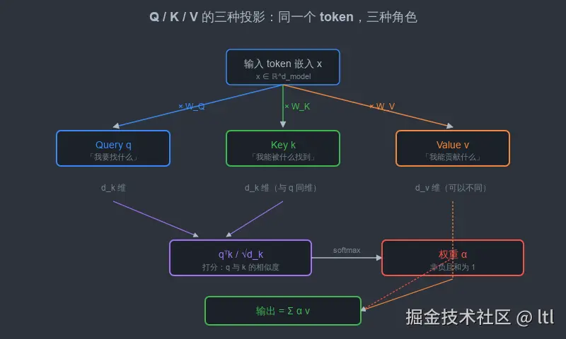
3.1 三种角色

把同一个 token <math xmlns="http://www.w3.org/1998/Math/MathML"> x x </math>x 投影成 <math xmlns="http://www.w3.org/1998/Math/MathML"> q q </math>q、 <math xmlns="http://www.w3.org/1998/Math/MathML"> k k </math>k、 <math xmlns="http://www.w3.org/1998/Math/MathML"> v v </math>v 三份，可以理解为给它戴上三顶帽子：

戴 Query 帽：「我此刻在找什么样的信息？」
戴 Key 帽：「我能被什么样的提问命中？」
戴 Value 帽：「如果被命中，我能贡献什么内容？」

这三个问题在语义上完全不同。

举个例子，当前 token 是「sat」（动词）。

它当 Query 时可能在找主语（「谁在 sat」），所以 <math xmlns="http://www.w3.org/1998/Math/MathML"> q q </math>q 应该编码一种「主语指向」的信号。

它当 Key 时可能希望被「找动词」的提问命中，所以 <math xmlns="http://www.w3.org/1998/Math/MathML"> k k </math>k 应该编码「我是动词」的信号。

它当 Value 时贡献的是「这个动作的语义」，所以 <math xmlns="http://www.w3.org/1998/Math/MathML"> v v </math>v 应该编码动作的具体信息（时态、语态、语义角色等）。

<math xmlns="http://www.w3.org/1998/Math/MathML"> W Q W_Q </math>WQ、 <math xmlns="http://www.w3.org/1998/Math/MathML"> W K W_K </math>WK、 <math xmlns="http://www.w3.org/1998/Math/MathML"> W V W_V </math>WV 就是把同一个 <math xmlns="http://www.w3.org/1998/Math/MathML"> x x </math>x 拉到这三种语义空间的三个投影。

3.2 投影矩阵学到了什么

这是经验观察，不是定理：

<math xmlns="http://www.w3.org/1998/Math/MathML"> W Q W_Q </math>WQ 学到的方向常常对应「这个 token 在找什么」------比如代词「it」的 <math xmlns="http://www.w3.org/1998/Math/MathML"> W Q W_Q </math>WQ 行为强烈倾向于找「最近的、可指代的名词」。
<math xmlns="http://www.w3.org/1998/Math/MathML"> W K W_K </math>WK 学到的方向常常对应「这个 token 适合被什么找到」------名词的 <math xmlns="http://www.w3.org/1998/Math/MathML"> W K W_K </math>WK 容易被指代代词找到、动词的 <math xmlns="http://www.w3.org/1998/Math/MathML"> W K W_K </math>WK 容易被主语/宾语找到。
<math xmlns="http://www.w3.org/1998/Math/MathML"> W V W_V </math>WV 学到的内容更接近「token 的语义指纹」------既要能被加权求和，又要在多层叠加下保持信息可分。

不同 head（multi-head attention）会学到不同的 <math xmlns="http://www.w3.org/1998/Math/MathML"> W Q / W K / W V W_Q/W_K/W_V </math>WQ/WK/WV，对应不同的「语法/语义关注模式」------有的 head 专门做指代消解，有的 head 专门做语法依存，有的 head 专门做局部上下文。

到第十六篇 multi-head 那里我们会把这件事拆开讲。

3.3 为什么是「投影」而不是别的非线性

<math xmlns="http://www.w3.org/1998/Math/MathML"> Q / K / V Q/K/V </math>Q/K/V 的投影是线性的（ <math xmlns="http://www.w3.org/1998/Math/MathML"> W Q ⋅ x W_Q \cdot x </math>WQ⋅x，没有激活函数），这是个有趣的设计选择。

Bahdanau 是非线性的（ <math xmlns="http://www.w3.org/1998/Math/MathML"> tanh ⁡ \tanh </math>tanh），Transformer 是线性的（直接矩阵乘）。

线性投影的好处：

计算便宜、GPU 极友好；
多层堆叠时，前一层的非线性（FFN 里的 ReLU/GeLU）已经提供了表达力；
投影后 <math xmlns="http://www.w3.org/1998/Math/MathML"> q ⋅ k q \cdot k </math>q⋅k 是双线性（关于 <math xmlns="http://www.w3.org/1998/Math/MathML"> q q </math>q 和 <math xmlns="http://www.w3.org/1998/Math/MathML"> k k </math>k 都是线性），变量分离让分析更容易。

代价：单层的 <math xmlns="http://www.w3.org/1998/Math/MathML"> Q / K / V Q/K/V </math>Q/K/V 投影本身没有非线性，所有非线性来自 FFN 模块。

Vaswani 等人的设计逻辑：「让 attention 专心做加权和、把非线性留给 FFN」------一种功能拆分。

到第二十篇 Transformer 整体架构那里，这种拆分会被重新强调。

四、公式逐项拆解

把主公式贴回来：
<math xmlns="http://www.w3.org/1998/Math/MathML" display="block"> Attention ( Q , K , V ) = softmax ( Q K ⊤ d k ) V \text{Attention}(Q, K, V) = \text{softmax}\left(\frac{QK^\top}{\sqrt{d_k}}\right) V </math>Attention(Q,K,V)=softmax(dk QK⊤)V

4.1 形状


Q	N × d_k
K	M × d_k
V	M × d_v
<math xmlns="http://www.w3.org/1998/Math/MathML"> Q K ⊤ QK^\top </math>QK⊤	N × M
<math xmlns="http://www.w3.org/1998/Math/MathML"> softmax ⁡ ( Q K ⊤ / d k ) \operatorname{softmax}(QK^\top / \sqrt{d_k}) </math>softmax(QK⊤/dk )	N × M（每行和=1）
Output	N × d_v

N = query 的个数；M = key/value 的个数；d_k = query/key 的维度；d_v = value 的维度。

cross-attention 时，N 和 M 可以不同（decoder 长度 vs encoder 长度）。

self-attention 时，N = M。

实践中，d_k 和 d_v 几乎总是相等（都等于 d_model / h，h 是 head 数）。

4.2 <math xmlns="http://www.w3.org/1998/Math/MathML"> Q K ⊤ QK^\top </math>QK⊤：所有 query 跟所有 key 的两两点积

<math xmlns="http://www.w3.org/1998/Math/MathML"> Q K ⊤ QK^\top </math>QK⊤ 这个操作是 attention 的灵魂。

直觉：把每个 query 跟每个 key 内积一次，得到 N×M 的「相似度矩阵」。

第 i 行第 j 列的元素 <math xmlns="http://www.w3.org/1998/Math/MathML"> ( Q K ⊤ ) i j = q i ⋅ k j (QK^\top)_{ij} = q_i \cdot k_j </math>(QK⊤)ij=qi⋅kj，表示「第 i 个 query 与第 j 个 key 的相似度」。

为什么用内积？

第一，便宜------一次矩阵乘搞定所有两两相似度，GPU 极快。

第二，几何意义清楚------内积 = 模长 × 模长 × cos 夹角，是「方向匹配 + 强度匹配」的自然组合。

第三，线性可微------对 q、k 都是线性函数，反向传播简单。

代价：内积没有「对称的非线性融合」，表达力比 additive attention 弱（虽然实际任务上几乎追平）。

4.3 <math xmlns="http://www.w3.org/1998/Math/MathML"> / d k / \sqrt{d_k} </math>/dk ：那个看似奇怪的缩放

为什么除以 <math xmlns="http://www.w3.org/1998/Math/MathML"> d k \sqrt{d_k} </math>dk ？

简短答案：当 d_k 增大时，q 与 k 的内积方差也线性增大；不缩放会导致 softmax 进入饱和区，梯度趋零。

详细推导留到下一篇（第十五篇），那里会用「两个 iid 单位方差向量内积的方差等于 d_k」这个事实正面推一遍。

这里你需要记住的是：<math xmlns="http://www.w3.org/1998/Math/MathML"> d k \sqrt{d_k} </math>dk 不是装饰，缺了它，d_k=64/128 这种规模的 attention 根本训不起来。

4.4 `softmax`：把分数变成权重分布

softmax 沿 N×M 矩阵的最后一维（也就是 M 维，每个 query 对所有 key 的分数）取，每一行都归一化为一个分布。

输出仍然是 N×M，但每行和为 1，每个元素 ∈ [0, 1]。

softmax 给我们带来三件好东西：

第一，所有 value 都被加权------没有信息被「argmax 砍掉」，hard alignment 学不到的多对一/多对多关系都能被表达。

第二，可微------softmax 是平滑函数，反向传播没有不连续点。

第三，自动归一 ------和为 1 让输出 <math xmlns="http://www.w3.org/1998/Math/MathML"> = ∑ i α i v i = \sum_i \alpha_i v_i </math>=∑iαivi 在数值范围上稳定，不会随 M 爆炸。

代价：softmax 有「赢者通吃」的倾向。当某个分数远高于其它时，对应权重接近 1，其它接近 0。这件事在「分数差异不大时」会让 attention 变得几乎均匀（等权），有时不够 sharp。

这是 sparsemax（Martins 2016）等替代方案出现的动机，但实践中 softmax 仍然是默认选择。

4.5 <math xmlns="http://www.w3.org/1998/Math/MathML"> ⋅ V \cdot V </math>⋅V：加权求和

最后一步是矩阵乘法：
<math xmlns="http://www.w3.org/1998/Math/MathML" display="block"> ( N × M ) ⋅ ( M × d v ) = ( N × d v ) (N \times M) \cdot (M \times d_v) = (N \times d_v) </math>(N×M)⋅(M×dv)=(N×dv)

每一行对应一个 query 的输出，是所有 value 按本行权重的加权平均。

直觉：「这个 query 此刻看 source（或 self）时，得到的混合信息」。

到这里 attention 就算完了。

整套流程：投影出 <math xmlns="http://www.w3.org/1998/Math/MathML"> Q / K / V Q/K/V </math>Q/K/V → 算两两相似度 → 缩放 → softmax → 加权求和。

简洁得几乎不像深度学习------它更像一个「可微的检索」。

五、维度走一遍：把所有矩阵乘法的形状都对一对

为了让公式真正「立」起来，我们用一组具体数字走一次整个流程。

设输入序列长度 <math xmlns="http://www.w3.org/1998/Math/MathML"> L = 8 L = 8 </math>L=8， <math xmlns="http://www.w3.org/1998/Math/MathML"> d m o d e l = 64 d_{model} = 64 </math>dmodel=64，head 数 <math xmlns="http://www.w3.org/1998/Math/MathML"> h = 8 h = 8 </math>h=8，每个 head 的 <math xmlns="http://www.w3.org/1998/Math/MathML"> d k = d v = 64 / 8 = 8 d_k = d_v = 64/8 = 8 </math>dk=dv=64/8=8。

5.1 单 head 的形状

输入 <math xmlns="http://www.w3.org/1998/Math/MathML"> X X </math>X： <math xmlns="http://www.w3.org/1998/Math/MathML"> L × d m o d e l = 8 × 64 L \times d_{model} = 8 \times 64 </math>L×dmodel=8×64

投影矩阵：

<math xmlns="http://www.w3.org/1998/Math/MathML"> W Q : d m o d e l × d k = 64 × 8 W_Q: d_{model} \times d_k = 64 \times 8 </math>WQ:dmodel×dk=64×8
<math xmlns="http://www.w3.org/1998/Math/MathML"> W K : d m o d e l × d k = 64 × 8 W_K: d_{model} \times d_k = 64 \times 8 </math>WK:dmodel×dk=64×8
<math xmlns="http://www.w3.org/1998/Math/MathML"> W V : d m o d e l × d v = 64 × 8 W_V: d_{model} \times d_v = 64 \times 8 </math>WV:dmodel×dv=64×8

投影后：

<math xmlns="http://www.w3.org/1998/Math/MathML"> Q = X ⋅ W Q : 8 × 8 Q = X \cdot W_Q: 8 \times 8 </math>Q=X⋅WQ:8×8
<math xmlns="http://www.w3.org/1998/Math/MathML"> K = X ⋅ W K : 8 × 8 K = X \cdot W_K: 8 \times 8 </math>K=X⋅WK:8×8
<math xmlns="http://www.w3.org/1998/Math/MathML"> V = X ⋅ W V : 8 × 8 V = X \cdot W_V: 8 \times 8 </math>V=X⋅WV:8×8

打分：

<math xmlns="http://www.w3.org/1998/Math/MathML"> Q K ⊤ QK^\top </math>QK⊤: <math xmlns="http://www.w3.org/1998/Math/MathML"> 8 × 8 8 \times 8 </math>8×8
缩放后仍 <math xmlns="http://www.w3.org/1998/Math/MathML"> 8 × 8 8 \times 8 </math>8×8
softmax 后仍 <math xmlns="http://www.w3.org/1998/Math/MathML"> 8 × 8 8 \times 8 </math>8×8（每行和 = 1）

加权求和：

<math xmlns="http://www.w3.org/1998/Math/MathML"> α ⋅ V : 8 × 8 \alpha \cdot V: 8 \times 8 </math>α⋅V:8×8

单 head 输出形状： <math xmlns="http://www.w3.org/1998/Math/MathML"> 8 × 8 8 \times 8 </math>8×8（与 <math xmlns="http://www.w3.org/1998/Math/MathML"> X X </math>X 的 <math xmlns="http://www.w3.org/1998/Math/MathML"> d m o d e l = 64 d_{model} = 64 </math>dmodel=64 不同！）

5.2 多 head 的拼接

multi-head 把 <math xmlns="http://www.w3.org/1998/Math/MathML"> h h </math>h 个 head 的输出沿最后一维 concat：

concat 后： <math xmlns="http://www.w3.org/1998/Math/MathML"> 8 × ( 8 ⋅ 8 ) = 8 × 64 8 \times (8 \cdot 8) = 8 \times 64 </math>8×(8⋅8)=8×64

再过一个输出投影：

<math xmlns="http://www.w3.org/1998/Math/MathML"> W O : d m o d e l × d m o d e l = 64 × 64 W_O: d_{model} \times d_{model} = 64 \times 64 </math>WO:dmodel×dmodel=64×64
最终输出： <math xmlns="http://www.w3.org/1998/Math/MathML"> ( 8 × 64 ) ⋅ ( 64 × 64 ) = 8 × 64 (8 \times 64) \cdot (64 \times 64) = 8 \times 64 </math>(8×64)⋅(64×64)=8×64

终于回到 <math xmlns="http://www.w3.org/1998/Math/MathML"> d m o d e l d_{model} </math>dmodel 维度，与输入 <math xmlns="http://www.w3.org/1998/Math/MathML"> X X </math>X 形状一致------可以接入残差连接。

5.3 batch 维度

实际训练时， <math xmlns="http://www.w3.org/1998/Math/MathML"> X X </math>X 形状是 <math xmlns="http://www.w3.org/1998/Math/MathML"> ( B , L , d m o d e l ) (B, L, d_{model}) </math>(B,L,dmodel)， <math xmlns="http://www.w3.org/1998/Math/MathML"> B B </math>B 是 batch 大小。

所有矩阵乘法都加一个 batch 维度做 broadcast： <math xmlns="http://www.w3.org/1998/Math/MathML"> ( B , L , d k ) ⋅ ( B , d k , L ) → ( B , L , L ) (B, L, d_k) \cdot (B, d_k, L) \to (B, L, L) </math>(B,L,dk)⋅(B,dk,L)→(B,L,L)。

PyTorch 的 torch.matmul 自动处理 batch；einops 库可以让形状操作更可读。

5.4 cross-attention 时的形状不对称

cross-attention 里， <math xmlns="http://www.w3.org/1998/Math/MathML"> Q Q </math>Q 来自 decoder， <math xmlns="http://www.w3.org/1998/Math/MathML"> K / V K/V </math>K/V 来自 encoder：

<math xmlns="http://www.w3.org/1998/Math/MathML"> Q : B × L t g t × d k Q: B \times L_{tgt} \times d_k </math>Q:B×Ltgt×dk
<math xmlns="http://www.w3.org/1998/Math/MathML"> K , V : B × L s r c × d k K, V: B \times L_{src} \times d_k </math>K,V:B×Lsrc×dk

<math xmlns="http://www.w3.org/1998/Math/MathML"> Q K ⊤ QK^\top </math>QK⊤: <math xmlns="http://www.w3.org/1998/Math/MathML"> B × L t g t × L s r c B \times L_{tgt} \times L_{src} </math>B×Ltgt×Lsrc，不再是方阵。

<math xmlns="http://www.w3.org/1998/Math/MathML"> L t g t L_{tgt} </math>Ltgt 和 <math xmlns="http://www.w3.org/1998/Math/MathML"> L s r c L_{src} </math>Lsrc 可以不同------这正是 attention 跨语言、跨模态的灵活性来源。

六、自注意力时的特殊性：Q/K/V 同源

self-attention 的特别之处在于 Q/K/V 都来自同一个输入 X：
<math xmlns="http://www.w3.org/1998/Math/MathML" display="block"> Q = X W Q K = X W K V = X W V \begin{aligned} Q &= X W_Q \\ K &= X W_K \\ V &= X W_V \end{aligned} </math>QKV=XWQ=XWK=XWV

虽然来源同源，但 <math xmlns="http://www.w3.org/1998/Math/MathML"> W Q W_Q </math>WQ、 <math xmlns="http://www.w3.org/1998/Math/MathML"> W K W_K </math>WK、 <math xmlns="http://www.w3.org/1998/Math/MathML"> W V W_V </math>WV 是三个独立学习的矩阵，所以 <math xmlns="http://www.w3.org/1998/Math/MathML"> Q ≠ K ≠ V Q \neq K \neq V </math>Q=K=V（一般情况下）。

这件事容易让人误以为 self-attention「让每个 token 跟自己最像」，但实际不是这样。

如果 <math xmlns="http://www.w3.org/1998/Math/MathML"> W Q = W K = I W_Q = W_K = I </math>WQ=WK=I（单位矩阵），那么 <math xmlns="http://www.w3.org/1998/Math/MathML"> q i ⊤ k j = x i ⊤ x j q_i^\top k_j = x_i^\top x_j </math>qi⊤kj=xi⊤xj，对角线（ <math xmlns="http://www.w3.org/1998/Math/MathML"> i = j i = j </math>i=j）确实最大。

但学过的 <math xmlns="http://www.w3.org/1998/Math/MathML"> W Q ≠ W K W_Q \neq W_K </math>WQ=WK 几乎总是把对角线打散，模型学到的注意力模式经常不是 self-loop 主导，而是「跨位置的语法/语义关联」。

「it」会强烈 attend「cat」，不是「it」自己；动词 attend 主语和宾语；定语 attend 中心词。

第 14 篇会把这件事讲得更具体。

七、玩具示例：3 token、d_k = 2，从头算到尾

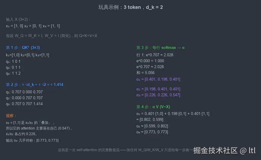
接下来是一个手算环节------这是这篇文章的核心实操段落。

7.1 设置

输入序列三个 token，每个嵌入向量 2 维：
<math xmlns="http://www.w3.org/1998/Math/MathML" display="block"> x 1 = [ 1 , 0 ] x 2 = [ 0 , 1 ] x 3 = [ 1 , 1 ] \begin{aligned} x_1 &= [1, 0] \\ x_2 &= [0, 1] \\ x_3 &= [1, 1] \end{aligned} </math>x1x2x3=[1,0]=[0,1]=[1,1]

为了简化，我们设 <math xmlns="http://www.w3.org/1998/Math/MathML"> W Q = W K = W V = I W_Q = W_K = W_V = I </math>WQ=WK=WV=I（单位矩阵），所以 <math xmlns="http://www.w3.org/1998/Math/MathML"> Q = K = V = X Q = K = V = X </math>Q=K=V=X。

实际模型当然不是单位矩阵，但这个简化让我们专注于「计算流」本身。

7.2 第一步： <math xmlns="http://www.w3.org/1998/Math/MathML"> Q K ⊤ QK^\top </math>QK⊤

<math xmlns="http://www.w3.org/1998/Math/MathML"> Q K ⊤ QK^\top </math>QK⊤ 是一个 <math xmlns="http://www.w3.org/1998/Math/MathML"> 3 × 3 3 \times 3 </math>3×3 矩阵，第 <math xmlns="http://www.w3.org/1998/Math/MathML"> ( i , j ) (i, j) </math>(i,j) 个元素是 <math xmlns="http://www.w3.org/1998/Math/MathML"> q i ⋅ k j q_i \cdot k_j </math>qi⋅kj：
<math xmlns="http://www.w3.org/1998/Math/MathML" display="block"> q 1 ⋅ k 1 = [ 1 , 0 ] ⋅ [ 1 , 0 ] = 1 q 1 ⋅ k 2 = [ 1 , 0 ] ⋅ [ 0 , 1 ] = 0 q 1 ⋅ k 3 = [ 1 , 0 ] ⋅ [ 1 , 1 ] = 1 q 2 ⋅ k 1 = [ 0 , 1 ] ⋅ [ 1 , 0 ] = 0 q 2 ⋅ k 2 = [ 0 , 1 ] ⋅ [ 0 , 1 ] = 1 q 2 ⋅ k 3 = [ 0 , 1 ] ⋅ [ 1 , 1 ] = 1 q 3 ⋅ k 1 = [ 1 , 1 ] ⋅ [ 1 , 0 ] = 1 q 3 ⋅ k 2 = [ 1 , 1 ] ⋅ [ 0 , 1 ] = 1 q 3 ⋅ k 3 = [ 1 , 1 ] ⋅ [ 1 , 1 ] = 2 \begin{aligned} q_1 \cdot k_1 &= [1,0]\cdot[1,0] = 1 \\ q_1 \cdot k_2 &= [1,0]\cdot[0,1] = 0 \\ q_1 \cdot k_3 &= [1,0]\cdot[1,1] = 1 \\[1ex] q_2 \cdot k_1 &= [0,1]\cdot[1,0] = 0 \\ q_2 \cdot k_2 &= [0,1]\cdot[0,1] = 1 \\ q_2 \cdot k_3 &= [0,1]\cdot[1,1] = 1 \\[1ex] q_3 \cdot k_1 &= [1,1]\cdot[1,0] = 1 \\ q_3 \cdot k_2 &= [1,1]\cdot[0,1] = 1 \\ q_3 \cdot k_3 &= [1,1]\cdot[1,1] = 2 \end{aligned} </math>q1⋅k1q1⋅k2q1⋅k3q2⋅k1q2⋅k2q2⋅k3q3⋅k1q3⋅k2q3⋅k3=[1,0]⋅[1,0]=1=[1,0]⋅[0,1]=0=[1,0]⋅[1,1]=1=[0,1]⋅[1,0]=0=[0,1]⋅[0,1]=1=[0,1]⋅[1,1]=1=[1,1]⋅[1,0]=1=[1,1]⋅[0,1]=1=[1,1]⋅[1,1]=2

矩阵形式：
<math xmlns="http://www.w3.org/1998/Math/MathML" display="block"> Q K ⊤ = [ 1 0 1 0 1 1 1 1 2 ] QK^\top = \begin{bmatrix} 1 & 0 & 1 \\ 0 & 1 & 1 \\ 1 & 1 & 2 \end{bmatrix} </math>QK⊤= 101011112

观察： <math xmlns="http://www.w3.org/1998/Math/MathML"> x 3 = x 1 + x 2 x_3 = x_1 + x_2 </math>x3=x1+x2，所以 <math xmlns="http://www.w3.org/1998/Math/MathML"> q 3 q_3 </math>q3 与所有 <math xmlns="http://www.w3.org/1998/Math/MathML"> k k </math>k 的相似度都更高，对角线 <math xmlns="http://www.w3.org/1998/Math/MathML"> q 3 ⋅ k 3 = 2 q_3 \cdot k_3 = 2 </math>q3⋅k3=2 是全场最大。

7.3 第二步：除以 <math xmlns="http://www.w3.org/1998/Math/MathML"> d k \sqrt{d_k} </math>dk = <math xmlns="http://www.w3.org/1998/Math/MathML"> 2 \sqrt{2} </math>2 ≈ 1.414

<math xmlns="http://www.w3.org/1998/Math/MathML" display="block"> [ 0.707 0.000 0.707 0.000 0.707 0.707 0.707 0.707 1.414 ] \begin{bmatrix} 0.707 & 0.000 & 0.707 \\ 0.000 & 0.707 & 0.707 \\ 0.707 & 0.707 & 1.414 \end{bmatrix} </math> 0.7070.0000.7070.0000.7070.7070.7070.7071.414

7.4 第三步：每行 softmax

<math xmlns="http://www.w3.org/1998/Math/MathML" display="block"> α 1 = softmax ⁡ ( [ 0.707 , 0.000 , 0.707 ] ) = [ e 0.707 e 0.707 + e 0 + e 0.707 , e 0 e 0.707 + e 0 + e 0.707 , e 0.707 e 0.707 + e 0 + e 0.707 ] ≈ [ 2.028 5.056 , 1.000 5.056 , 2.028 5.056 ] ≈ [ 0.401 , 0.198 , 0.401 ] \begin{aligned} \alpha_1 &= \operatorname{softmax}([0.707, 0.000, 0.707]) \\ &= \left[\frac{e^{0.707}}{e^{0.707}+e^{0}+e^{0.707}},\; \frac{e^{0}}{e^{0.707}+e^{0}+e^{0.707}},\; \frac{e^{0.707}}{e^{0.707}+e^{0}+e^{0.707}}\right] \\ &\approx \left[\frac{2.028}{5.056},\; \frac{1.000}{5.056},\; \frac{2.028}{5.056}\right] \\ &\approx [0.401,\; 0.198,\; 0.401] \end{aligned} </math>α1=softmax([0.707,0.000,0.707])=[e0.707+e0+e0.707e0.707,e0.707+e0+e0.707e0,e0.707+e0+e0.707e0.707]≈[5.0562.028,5.0561.000,5.0562.028]≈[0.401,0.198,0.401]
<math xmlns="http://www.w3.org/1998/Math/MathML" display="block"> α 2 = softmax ⁡ ( [ 0.000 , 0.707 , 0.707 ] ) ≈ [ 0.198 , 0.401 , 0.401 ] \alpha_2 = \operatorname{softmax}([0.000, 0.707, 0.707]) \approx [0.198,\; 0.401,\; 0.401] </math>α2=softmax([0.000,0.707,0.707])≈[0.198,0.401,0.401]
<math xmlns="http://www.w3.org/1998/Math/MathML" display="block"> α 3 = softmax ⁡ ( [ 0.707 , 0.707 , 1.414 ] ) = [ e 0.707 e 0.707 + e 0.707 + e 1.414 , e 0.707 e 0.707 + e 0.707 + e 1.414 , e 1.414 e 0.707 + e 0.707 + e 1.414 ] ≈ [ 2.028 8.169 , 2.028 8.169 , 4.113 8.169 ] ≈ [ 0.248 , 0.248 , 0.503 ] \begin{aligned} \alpha_3 &= \operatorname{softmax}([0.707, 0.707, 1.414]) \\ &= \left[\frac{e^{0.707}}{e^{0.707}+e^{0.707}+e^{1.414}},\; \frac{e^{0.707}}{e^{0.707}+e^{0.707}+e^{1.414}},\; \frac{e^{1.414}}{e^{0.707}+e^{0.707}+e^{1.414}}\right] \\ &\approx \left[\frac{2.028}{8.169},\; \frac{2.028}{8.169},\; \frac{4.113}{8.169}\right] \\ &\approx [0.248,\; 0.248,\; 0.503] \end{aligned} </math>α3=softmax([0.707,0.707,1.414])=[e0.707+e0.707+e1.414e0.707,e0.707+e0.707+e1.414e0.707,e0.707+e0.707+e1.414e1.414]≈[8.1692.028,8.1692.028,8.1694.113]≈[0.248,0.248,0.503]

（注：我用更精确的数取整，写得更细致；论文里通常给三位有效数字。）

7.5 第四步：α · V（V = X）

<math xmlns="http://www.w3.org/1998/Math/MathML" display="block"> o 1 = 0.401 ⋅ [ 1 , 0 ] + 0.198 ⋅ [ 0 , 1 ] + 0.401 ⋅ [ 1 , 1 ] = [ 0.401 , 0 ] + [ 0 , 0.198 ] + [ 0.401 , 0.401 ] = [ 0.802 , 0.599 ] o 2 = 0.198 ⋅ [ 1 , 0 ] + 0.401 ⋅ [ 0 , 1 ] + 0.401 ⋅ [ 1 , 1 ] = [ 0.599 , 0.802 ] o 3 = 0.248 ⋅ [ 1 , 0 ] + 0.248 ⋅ [ 0 , 1 ] + 0.503 ⋅ [ 1 , 1 ] = [ 0.751 , 0.751 ] \begin{aligned} o_1 &= 0.401 \cdot [1,0] + 0.198 \cdot [0,1] + 0.401 \cdot [1,1] \\ &= [0.401, 0] + [0, 0.198] + [0.401, 0.401] \\ &= [0.802, 0.599] \\[1ex] o_2 &= 0.198 \cdot [1,0] + 0.401 \cdot [0,1] + 0.401 \cdot [1,1] \\ &= [0.599, 0.802] \\[1ex] o_3 &= 0.248 \cdot [1,0] + 0.248 \cdot [0,1] + 0.503 \cdot [1,1] \\ &= [0.751, 0.751] \end{aligned} </math>o1o2o3=0.401⋅[1,0]+0.198⋅[0,1]+0.401⋅[1,1]=[0.401,0]+[0,0.198]+[0.401,0.401]=[0.802,0.599]=0.198⋅[1,0]+0.401⋅[0,1]+0.401⋅[1,1]=[0.599,0.802]=0.248⋅[1,0]+0.248⋅[0,1]+0.503⋅[1,1]=[0.751,0.751]

最终输出三个新 token：
<math xmlns="http://www.w3.org/1998/Math/MathML" display="block"> o 1 ≈ [ 0.802 , 0.599 ] o 2 ≈ [ 0.599 , 0.802 ] o 3 ≈ [ 0.751 , 0.751 ] \begin{aligned} o_1 &\approx [0.802, 0.599] \\ o_2 &\approx [0.599, 0.802] \\ o_3 &\approx [0.751, 0.751] \end{aligned} </math>o1o2o3≈[0.802,0.599]≈[0.599,0.802]≈[0.751,0.751]

7.6 观察

第一，o_1 和 o_2 不对称：o_1 第一维更大（因为 x_1 主导），o_2 第二维更大（因为 x_2 主导）。

这说明 self-attention 让每个 token 仍然保留了自己的「身份」，但混入了与其它 token 的相关信息。

第二，o_3 几乎对称：[0.751, 0.751]，因为 x_3 跟 x_1、x_2 都同等相关，所以加权和被「抹平」了。

第三，所有输出向量都比输入「更接近彼此」------self-attention 是一种信息融合操作，会让 token 之间的差异减小。

这是为什么 Transformer 要堆 N 层 self-attention：单层的「融合」不够，需要多层迭代地把信息打散又重组。

7.7 把 W_Q/W_K/W_V 加进来会发生什么

如果 W_Q ≠ W_K（即使都是随机的小矩阵），上面的 <math xmlns="http://www.w3.org/1998/Math/MathML"> Q K T QK^T </math>QKT 矩阵会变样------可能 q_3·k_3 不再最大，可能某个 (i, j) 跨位置的相似度反而最高。

这就是模型「学」出来的注意力模式：不再是「自己最像自己」，而是「按学到的语义匹配」。

到第十四篇我们会用一个真实例子（"The cat sat on the mat. It was tired."）演示这件事。

八、Additive 还是 Multiplicative：scaled dot-product 为什么赢

第 12 篇里讨论过 additive (Bahdanau) vs multiplicative (Luong) 的区别。

到 Transformer 时代，scaled dot-product attention（multiplicative 的一种）成为绝对主流。

为什么？

8.1 GPU 友好

<math xmlns="http://www.w3.org/1998/Math/MathML"> Q K T QK^T </math>QKT 是一个矩阵乘法，可以用 cuBLAS、cuDNN、TensorCore 等加速到极致。

additive attention 需要逐对算 <math xmlns="http://www.w3.org/1998/Math/MathML"> v ⊤ tanh ⁡ ( W 1 q + W 2 k ) v^\top \tanh(W_1 q + W_2 k) </math>v⊤tanh(W1q+W2k)------虽然也可以批处理，但常数开销大、内存访问模式不规则。

在 d_k = 64 的规模下，scaled dot-product 的速度大约是 additive 的 3-5 倍（不带 <math xmlns="http://www.w3.org/1998/Math/MathML"> d k \sqrt{d_k} </math>dk 缩放时）。

8.2 参数更少

additive： <math xmlns="http://www.w3.org/1998/Math/MathML"> W 1 ∈ R d × d q W_1 \in \mathbb{R}^{d \times d_q} </math>W1∈Rd×dq， <math xmlns="http://www.w3.org/1998/Math/MathML"> W 2 ∈ R d × d k W_2 \in \mathbb{R}^{d \times d_k} </math>W2∈Rd×dk， <math xmlns="http://www.w3.org/1998/Math/MathML"> v ∈ R d v \in \mathbb{R}^{d} </math>v∈Rd，三组参数。

scaled dot-product：W_Q、W_K、W_V，但 W_Q/W_K/W_V 在多头里也是 query/key/value 的投影矩阵------它们的参数会被 multi-head 复用。

实际比较时，scaled dot-product 的「打分专用参数」是 0（投影本身已经摊销在 Q/K/V 的生成里）。

8.3 在大 d_k 下，缩放后差距小

Vaswani 2017 论文 §3.2.1 直接对比了 additive 和 dot-product。

不带 <math xmlns="http://www.w3.org/1998/Math/MathML"> d k \sqrt{d_k} </math>dk 缩放时，dot-product 在 d_k 大时显著差于 additive（softmax 饱和）。

加了 <math xmlns="http://www.w3.org/1998/Math/MathML"> d k \sqrt{d_k} </math>dk 缩放后，两者性能接近，但 dot-product 速度快得多。

这就是 Transformer 选 scaled dot-product 的核心论点：性能接近，速度更快，参数更少。

8.4 Additive 还活着的场景

不要以为 additive 已死。

第 12 篇里讲过，Tacotron、pointer networks、GAT（Graph Attention Network）这些场景仍然广泛使用 additive。

原因主要是：小模型 + 短序列 + 强先验需求时，additive 的稳定性更好。

到 LLM 规模才需要 scaled dot-product 的所有优势。

九、几个常被忽略的细节

9.1 W_Q/W_K/W_V 的初始化

实践中，W_Q/W_K/W_V 用 Xavier（Glorot）初始化或 Kaiming 初始化。

不能用全零------会让所有 q/k 都是零向量， <math xmlns="http://www.w3.org/1998/Math/MathML"> Q K T QK^T </math>QKT 全零，softmax 退化成均匀分布。

不能用过大方差------会让 q·k 的方差远超 d_k，softmax 立刻饱和。

Vaswani 2017 用的是 fan_in 标准差的 Xavier，配合 <math xmlns="http://www.w3.org/1998/Math/MathML"> d k \sqrt{d_k} </math>dk 缩放，让训练初期 softmax 输入接近 N(0, 1)。

9.2 在多 head 情形下，W_Q 的「真实形状」

很多教材写 W_Q ∈ ℝ^{d_model × d_k}（单 head），但实际实现里 W_Q 是 ℝ^{d_model × d_model}：

d_model = h × d_k；
W_Q 是把所有 h 个 head 的投影矩阵拼在一起的一个大矩阵；
投影后 reshape 成 (B, L, h, d_k)，再 transpose 成 (B, h, L, d_k) 进 attention。

这样实现的好处：一次矩阵乘搞定 h 个 head 的投影，不用循环。

PyTorch 的 nn.MultiheadAttention 内部就是这么做的。

9.3 attention 不是单射

注意：从 (Q, K, V) 到 attention 的输出，是一个满射而不是单射。

不同的 (Q, K, V) 可以产生相同的 output（α 的对称性、value 的可加性）。

也就是说，attention 输出本身丢失了一些信息------所以 Transformer 要靠残差连接保住原始输入。

去掉残差后 Transformer 几乎训不起来------这是经验法则，不是理论必然。

9.4 Numerical stability：log-sum-exp trick

<math xmlns="http://www.w3.org/1998/Math/MathML"> softmax ⁡ ( x i ) = exp ⁡ ( x i ) / ∑ j exp ⁡ ( x j ) \operatorname{softmax}(x_i) = \exp(x_i) / \sum_j \exp(x_j) </math>softmax(xi)=exp(xi)/∑jexp(xj) 在 <math xmlns="http://www.w3.org/1998/Math/MathML"> x i x_i </math>xi 很大时会数值溢出。

实现时通常用 log-sum-exp trick：先把所有 x_i 减去 max(x)，再 softmax。

这件事每个深度学习框架都自动处理，但你写自定义 attention（比如调试自定义 mask）时要记得。

9.5 Mask 怎么加进 attention

causal mask（防止看到未来）通常通过把对应位置的 score 设为 <math xmlns="http://www.w3.org/1998/Math/MathML"> − ∞ -\infty </math>−∞ 实现：
<math xmlns="http://www.w3.org/1998/Math/MathML" display="block"> S = Q K ⊤ d k S i j = − ∞ （mask 位置） α = softmax ⁡ ( S ) \begin{aligned} S &= \frac{QK^\top}{\sqrt{d_k}} \\ S_{ij} &= -\infty \quad \text{（mask 位置）} \\ \alpha &= \operatorname{softmax}(S) \end{aligned} </math>SSijα=dk QK⊤=−∞（mask 位置）=softmax(S)

<math xmlns="http://www.w3.org/1998/Math/MathML"> softmax ⁡ ( − ∞ ) = 0 \operatorname{softmax}(-\infty) = 0 </math>softmax(−∞)=0，所以 mask 位置的权重为零。

这件事到第十七篇 causal mask 那里会专门讲。

十、一些 attention 的「不变量」

无论 attention 怎么变，下面几件事永远成立：

第一，softmax 输出一定是一个概率分布------非负、和为 1。

第二，输出 <math xmlns="http://www.w3.org/1998/Math/MathML"> = ∑ i α i v i = \sum_i \alpha_i v_i </math>=∑iαivi ，输出的 <math xmlns="http://www.w3.org/1998/Math/MathML"> d v d_v </math>dv 维度等于 V 的 <math xmlns="http://www.w3.org/1998/Math/MathML"> d v d_v </math>dv。

第三，改变 query 顺序，不影响其它 query 的输出------attention 沿 query 轴是 row-wise 独立的。

第四，改变 key/value 的顺序（同步改），不影响最终输出------attention 关于 (key, value) 的排列是不变的（permutation-equivariant）。

第三、第四点合起来：attention 本身不知道位置。这正是 Transformer 必须配位置编码的原因------下一节、下一篇会反复讲。

十一、一个常见的实现陷阱： <math xmlns="http://www.w3.org/1998/Math/MathML"> Q K ⊤ QK^\top </math>QK⊤ 的内存

<math xmlns="http://www.w3.org/1998/Math/MathML"> Q K ⊤ QK^\top </math>QK⊤ 的形状是 <math xmlns="http://www.w3.org/1998/Math/MathML"> ( B , h , N , M ) (B, h, N, M) </math>(B,h,N,M)。

当 <math xmlns="http://www.w3.org/1998/Math/MathML"> N = M = L N = M = L </math>N=M=L（self-attention）且 <math xmlns="http://www.w3.org/1998/Math/MathML"> L = 8192 L = 8192 </math>L=8192 时，单个 head 的 <math xmlns="http://www.w3.org/1998/Math/MathML"> Q K ⊤ QK^\top </math>QK⊤ 矩阵是 <math xmlns="http://www.w3.org/1998/Math/MathML"> 8192 × 8192 = 6700 8192 \times 8192 = 6700 </math>8192×8192=6700 万个 float，单 head 仅需 256 MB（fp32）；32 head 一起就是 8 GB。

这就是 Transformer 在长上下文下「显存爆炸」的来源------ <math xmlns="http://www.w3.org/1998/Math/MathML"> Q K ⊤ QK^\top </math>QK⊤ 矩阵本身的大小是 <math xmlns="http://www.w3.org/1998/Math/MathML"> O ( L 2 ) O(L^2) </math>O(L2)。

FlashAttention（Dao et al. 2022）的核心 trick 就是不显式存储 <math xmlns="http://www.w3.org/1998/Math/MathML"> Q K ⊤ QK^\top </math>QK⊤ ，而是把它分块、流式地计算 softmax 和加权和，避免把 <math xmlns="http://www.w3.org/1998/Math/MathML"> N × M N \times M </math>N×M 矩阵写到显存。

到第十八篇 attention 复杂度那里会讨论这件事。

但现在你需要知道的是： <math xmlns="http://www.w3.org/1998/Math/MathML"> Q K ⊤ QK^\top </math>QK⊤ 的存在让 attention 在长序列上不便宜------这是后续所有「线性 attention」「稀疏 attention」研究的原始动机。

十二、几种常见的「Q/K/V 变体」速览

主公式只有一种，但围绕它衍生出大量变体。这一节用最短篇幅勾勒几个高频名字，让你后面看论文时不发懵。

12.1 Multi-Query / Grouped-Query Attention

标准 Transformer 里每个 head 都有自己的 K、V。

Multi-Query Attention（MQA, Shazeer 2019）让所有 head 共享同一组 K、V，只 query 各自不同。

参数减少 h 倍，KV cache 也减少 h 倍------推理时极其重要。

代价是表达力略降。

Grouped-Query Attention（GQA, Ainslie 2023）是折中方案：把 h 个 head 分成 g 组，每组共享一份 K/V。

LLaMA-2 70B、Mistral 7B 等都在用 GQA。

到 2026 年，几乎所有大模型推理时都至少用 GQA，纯 MHA 已经退出大模型设计。

12.2 Cross-Attention

Q 来自一个序列，K/V 来自另一个序列。

经典场景：

机器翻译 decoder：Q 来自目标语言，K/V 来自源语言；
T5、BART 等 encoder-decoder 模型；
多模态：Q 来自文本，K/V 来自图像（或反之）；
Stable Diffusion 的 U-Net 里 text → image 的 cross-attention。

cross-attention 在 Q/K/V 框架里只是「Q 和 K/V 来源不同」这一件事，公式完全不变。

12.3 Encoder-only Self-Attention

BERT 类模型只有 encoder，里面是双向 self-attention：每个 token 可以 attend 所有 token（包括未来）。

没有 causal mask，因此可以并行做完整双向上下文建模。

代价：不能用来做生成（看到了未来 token）。

12.4 Decoder-only Causal Self-Attention

GPT 类模型只有 decoder，里面是 causal self-attention：每个 token 只能 attend 到自己和左侧。

通过加一个上三角的 -∞ mask 实现。

适合自回归生成。

到 2026 年，绝大多数大模型（GPT-4、Claude、Gemini、LLaMA、Qwen）都是 decoder-only 架构。

12.5 Linear / Kernel Attention

Performer（Choromanski 2020）、Linformer（Wang 2020）等把 <math xmlns="http://www.w3.org/1998/Math/MathML"> softmax ⁡ ( Q K ⊤ ) \operatorname{softmax}(QK^\top) </math>softmax(QK⊤) 近似成 <math xmlns="http://www.w3.org/1998/Math/MathML"> ϕ ( Q ) ϕ ( K ) ⊤ \phi(Q) \phi(K)^\top </math>ϕ(Q)ϕ(K)⊤，让 attention 退化成 <math xmlns="http://www.w3.org/1998/Math/MathML"> O ( N ) O(N) </math>O(N) 而不是 <math xmlns="http://www.w3.org/1998/Math/MathML"> O ( N 2 ) O(N^2) </math>O(N2)。

代价：精度损失，长序列上常见但 LLM 主流尚未采用。

12.6 Sliding Window / Local Attention

每个 query 只 attend 邻近 <math xmlns="http://www.w3.org/1998/Math/MathML"> W W </math>W 个 key（ <math xmlns="http://www.w3.org/1998/Math/MathML"> W ≪ N W \ll N </math>W≪N），复杂度是 <math xmlns="http://www.w3.org/1998/Math/MathML"> O ( N ⋅ W ) O(N \cdot W) </math>O(N⋅W)。

Longformer、Mistral 都用过这种结构。

12.7 Sparse Attention

按某种 pattern（块、稀疏、随机）让大部分 (i, j) 对被 mask 掉。

BigBird、Sparse Transformer 是代表。

复杂度可降到 <math xmlns="http://www.w3.org/1998/Math/MathML"> O ( N log ⁡ N ) O(N \log N) </math>O(NlogN) 或 <math xmlns="http://www.w3.org/1998/Math/MathML"> O ( N N ) O(N \sqrt{N}) </math>O(NN )。

12.8 Mixture of Attention Heads

不同输入用不同的 head（类似 MoE 那种 gating）。

代表：MoH（2024 年开始流行）。

十三、把 Q/K/V 写成 PyTorch 代码

光讲公式不够，看一段最简实现能让公式立得更稳。

下面是 self-attention（单 head）的最小可运行代码：

python 复制代码

import torch
import torch.nn as nn
import torch.nn.functional as F

class SelfAttention(nn.Module):
    def __init__(self, d_model, d_k):
        super().__init__()
        self.d_k = d_k
        self.W_Q = nn.Linear(d_model, d_k, bias=False)
        self.W_K = nn.Linear(d_model, d_k, bias=False)
        self.W_V = nn.Linear(d_model, d_k, bias=False)

    def forward(self, x, mask=None):
        # x: (B, L, d_model)
        Q = self.W_Q(x)                # (B, L, d_k)
        K = self.W_K(x)
        V = self.W_V(x)

        scores = Q @ K.transpose(-2, -1) / (self.d_k ** 0.5)  # (B, L, L)
        if mask is not None:
            scores = scores.masked_fill(mask == 0, float('-inf'))
        alpha = F.softmax(scores, dim=-1)
        out = alpha @ V                # (B, L, d_k)
        return out, alpha

这段代码就是 attention 的全部------加上残差、LayerNorm、FFN、multi-head 投影、causal mask 之后，就成了 Transformer。

你可以试着跑一下：

python 复制代码

torch.manual_seed(42)
attn = SelfAttention(d_model=8, d_k=8)
x = torch.randn(1, 5, 8)
out, alpha = attn(x)
print(alpha.shape)  # (1, 5, 5)
print(alpha.sum(dim=-1))  # 每行接近 1

第一次跑通这段代码，你对 attention 的直觉会从「公式上的事」变成「指尖上的事」。

13.1 工程实现里几个常见错误

第一，忘了 <math xmlns="http://www.w3.org/1998/Math/MathML"> d k \sqrt{d_k} </math>dk 。直接 Q @ K.transpose(-2, -1)， <math xmlns="http://www.w3.org/1998/Math/MathML"> d k = 64 d_k = 64 </math>dk=64 时基本训不起来。

第二，softmax 的轴搞错。要在「key 轴」（最后一维）上 softmax，不是在 query 轴。

第三，mask 的方向搞反 。causal mask 是「不能看到未来」，对应 mask 的上三角应该被填 <math xmlns="http://www.w3.org/1998/Math/MathML"> − ∞ -\infty </math>−∞。

第四，用 <math xmlns="http://www.w3.org/1998/Math/MathML"> m a s k = 0 \mathrm{mask}=0 </math>mask=0 表示「保留」、 <math xmlns="http://www.w3.org/1998/Math/MathML"> m a s k = 1 \mathrm{mask}=1 </math>mask=1 表示「屏蔽」时，masked_fill 要对应着写。PyTorch 默认 masked_fill(mask, value) 是「mask 为 True 的位置填 value」------容易写反。

第五，dropout 的位置 。Vaswani 原版在 softmax 后、加权和前对 <math xmlns="http://www.w3.org/1998/Math/MathML"> α \alpha </math>α 做 dropout。这个细节经常被省略，但会影响训练动力学。

十四、Q/K/V 的训练动态：模型怎么学到这三个矩阵

理论上 <math xmlns="http://www.w3.org/1998/Math/MathML"> W Q / W K / W V W_Q/W_K/W_V </math>WQ/WK/WV 是可学习参数，初始化时是随机的。

那模型怎么把它们「学」成有意义的语义投影？

14.1 起点：完全随机的 Q/K/V

训练初期， <math xmlns="http://www.w3.org/1998/Math/MathML"> W Q / W K / W V W_Q/W_K/W_V </math>WQ/WK/WV 都是随机小矩阵。

<math xmlns="http://www.w3.org/1998/Math/MathML"> Q K ⊤ QK^\top </math>QK⊤ 接近随机噪声，softmax 后 <math xmlns="http://www.w3.org/1998/Math/MathML"> α \alpha </math>α 几乎均匀（每个 query 对所有 key 大致等权）。

这时 attention 的输出 ≈ 所有 V 的均值------本质上是「每个 token 都在看所有 token 的平均」。

这件事看起来很糟糕，但实际上是合理的起点：模型先学到「token 的全局上下文均值」，然后逐步学会 sharpen attention。

14.2 中期：sharpening 与 specialization

随着训练进行，反向传播会推动 <math xmlns="http://www.w3.org/1998/Math/MathML"> W Q / W K / W V W_Q/W_K/W_V </math>WQ/WK/WV 朝「让 loss 下降」的方向更新。

这时模型开始发现：「对某些 query，应该 attend 到特定 key」会让预测更准。

<math xmlns="http://www.w3.org/1998/Math/MathML"> α \alpha </math>α 开始 sharpen------某些权重显著大于其它。

不同 head 开始 specialize：head 1 关注语法依存，head 3 关注共指消解，head 7 关注下一个 token------这些都是 BERT/GPT 训练后被实证观察到的模式。

14.3 末期：稳定的 attention pattern

充分训练后，每个 head 的 attention pattern 大致稳定。

不同输入会激活不同的 pattern，但每个 head 对「自己关注什么」是稳定的。

这种稳定性让 attention 可视化变得有意义------也是 BertViz、Attention is not Explanation 等可视化/解释工具的基础。

14.4 一些训练失败的模式

attention head collapse：所有 head 学到了几乎一样的 pattern。

attention oversmoothing：所有 token 的输出都趋同，模型失去区分能力。

attention degenerate to one position：所有 query 都 attend 到第一个或最后一个 token（通常是 BOS / EOS）。

这些都是真实存在的失败模式，到 LLM 工程实践里有专门技术（warmup 长度、label smoothing、gradient clipping、attention dropout）来缓解。

十五、关键概念回顾

走到这里，我们把 Q/K/V 拆得彻底了。最该带走的几句话：

Q/K/V 是软检索的三件套：Query 提问、Key 被打分、Value 被加权求和。

主公式 <math xmlns="http://www.w3.org/1998/Math/MathML"> Attention ( Q , K , V ) = softmax ( Q K ⊤ / d k ) V \text{Attention}(Q,K,V) = \text{softmax}(QK^\top/\sqrt{d_k}) V </math>Attention(Q,K,V)=softmax(QK⊤/dk )V 一行包含五件事：投影、内积打分、缩放、归一化、加权求和。

K 和 V 解耦让模型可以独立优化「索引」和「内容」------这是从 Bahdanau 到 Transformer 最关键的设计跳跃。

<math xmlns="http://www.w3.org/1998/Math/MathML"> W Q / W K / W V W_Q/W_K/W_V </math>WQ/WK/WV 是三个独立学习的线性投影，把同一个输入拉到三种不同的语义空间。

self-attention 时 Q/K/V 同源但形态不同------投影矩阵让「同一 token 的三种角色」可以分别学习。

<math xmlns="http://www.w3.org/1998/Math/MathML"> d k \sqrt{d_k} </math>dk 缩放是为了让 softmax 不饱和------缺了它，d_k 一上 64 训练就崩。

attention 不知道位置------它对 key/value 的排列等变，必须靠位置编码或 causal mask 注入位置信息。

十六、常见误解

13.1 Q/K/V 必须从同一个输入投影

不对。

cross-attention 里 Q 来自 decoder，K/V 来自 encoder，是两个不同输入。

「同源」是 self-attention 的特例。

13.2 K 和 V 可以省掉一个

不可以------除非你愿意接受 Bahdanau 的限制（K = V = h）。

K 和 V 解耦才让模型有能力区分「索引信号」和「内容信号」，省掉一个会显著降低表达力。

13.3 d_k 必须等于 d_v

不必。

虽然 Transformer 默认 d_k = d_v = d_model / h，但理论上 d_k 和 d_v 可以独立设。

实践中保持一致是为了简洁和参数对称。

13.4 attention 的本质是「相似度」

部分对。

<math xmlns="http://www.w3.org/1998/Math/MathML"> Q K ⊤ QK^\top </math>QK⊤ 是相似度，softmax 是归一化，但「Q/K/V 三件套」的本质更准确地说是软检索------不是单纯比相似度，而是「按相似度加权地从 Value 池里取信息」。

13.5 attention 是 O(1) 的

完全不对。

attention 是 <math xmlns="http://www.w3.org/1998/Math/MathML"> O ( N ⋅ M ⋅ d k ) O(N \cdot M \cdot d_k) </math>O(N⋅M⋅dk)（计算 <math xmlns="http://www.w3.org/1998/Math/MathML"> Q K ⊤ QK^\top </math>QK⊤） <math xmlns="http://www.w3.org/1998/Math/MathML"> + O ( N ⋅ M ⋅ d v ) +\;O(N \cdot M \cdot d_v) </math>+O(N⋅M⋅dv)（加权和），关于序列长度是平方复杂度。

「O(1) 路径长度」是另一回事------指任意两个 token 在一层内可以直接交互（不像 RNN 要走 N 步），这是「路径」上的 O(1)，不是「计算」上的 O(1)。

13.6 softmax 之前一定要除以 <math xmlns="http://www.w3.org/1998/Math/MathML"> d k \sqrt{d_k} </math>dk

几乎是的。

不除会让训练在 <math xmlns="http://www.w3.org/1998/Math/MathML"> d k > 16 d_k > 16 </math>dk>16 时基本崩溃。但有些工作（如 LayerNorm 在 score 上的 attention）可以代替缩放------这是变体，不是默认。

13.7 W_Q 和 W_K 是「对称」的

不是。

<math xmlns="http://www.w3.org/1998/Math/MathML"> W Q W_Q </math>WQ 学到的方向不等于 <math xmlns="http://www.w3.org/1998/Math/MathML"> W K W_K </math>WK 学到的方向。query 和 key 在同一 head 里学到的子空间可以差很远------这正是为什么模型能学到「跨语义」的 attention 模式。

13.8 KV cache 是 K 和 V 的简单缓存

部分对------KV cache 确实是把已经算过的 K、V 缓存下来，避免重复计算。

但「KV」这个名字常被误读为「Key-Value 数据库」------实际上它是 attention 里的 K 矩阵和 V 矩阵，与数据库 KV store 没有任何关系。

到第二十二篇 KV cache 那里我们会专门讲它的形状、占用与优化。

13.9 attention 输出维度等于 Q 的维度

不是。

attention 输出维度等于 <math xmlns="http://www.w3.org/1998/Math/MathML"> V V </math>V 的维度（ <math xmlns="http://www.w3.org/1998/Math/MathML"> d v d_v </math>dv）。

只是实践中 <math xmlns="http://www.w3.org/1998/Math/MathML"> d q = d k = d v d_q = d_k = d_v </math>dq=dk=dv 让人产生这个错觉。

如果你设 <math xmlns="http://www.w3.org/1998/Math/MathML"> d v ≠ d k d_v \neq d_k </math>dv=dk，attention 输出形状就会是 <math xmlns="http://www.w3.org/1998/Math/MathML"> ( N , d v ) (N, d_v) </math>(N,dv) 而不是 <math xmlns="http://www.w3.org/1998/Math/MathML"> ( N , d k ) (N, d_k) </math>(N,dk)。

十七、下一步

下一篇 14｜Self-Attention 会把 Q/K/V 框架进一步特化到「同一序列内 token 互相 attend」的情形。

我们会展示：

当 Q/K/V 都来自同一序列时，attention 退化成什么样子；
为什么 self-attention 能在 O(1) 跳数内让任意两 token 交互；
为什么它对位置完全无知------这是位置编码登场的原因；
一个具体例子：「The cat sat on the mat. It was tired.」中 "it" 怎么 attend 到 "cat"。

再往后：15｜Scaled Dot-Product 会用方差推导讲清 <math xmlns="http://www.w3.org/1998/Math/MathML"> d k \sqrt{d_k} </math>dk 这个奇怪的常数为什么必要。

第 16 篇会讲 multi-head------为什么一个 attention 不够，要 8 个或更多并行。

到时候你会看到：multi-head 不是「多算几遍取平均」，而是每个 head 学一个不同的 Q/K/V 子空间------这才是性能提升的真正来源。

如果你想动手验证今天讲的所有内容，最快的方式是：拿 PyTorch 写一个 SelfAttention 类（就是十三节的代码），用三 token、d_k=2 的输入跑一次，把每一步打印出来，跟手算的结果对一对。

只要数值能对上，你对 attention 的直觉就立住了------后面所有变种、所有论文，都只是这个基础上的加减法。

十八、参考文献

下面按相关度排序，列出本篇直接引用与延伸阅读，每条附一句话提示其在本篇中的角色。

Vaswani, A. et al. "Attention Is All You Need." NeurIPS 2017. Q/K/V 三件套与 scaled dot-product 公式的源头。
Bahdanau, D., Cho, K., Bengio, Y. "Neural Machine Translation by Jointly Learning to Align and Translate." ICLR 2015 (arXiv:1409.0473, 2014). Q/K/V 的「前身」------additive attention。
Luong, M.-T., Pham, H., Manning, C. D. "Effective Approaches to Attention-based Neural Machine Translation." EMNLP 2015. multiplicative attention 的代表，Vaswani 论文 §3.2.1 与之直接对照。
Dao, T. et al. "FlashAttention: Fast and Memory-Efficient Exact Attention with IO-Awareness." NeurIPS 2022 . <math xmlns="http://www.w3.org/1998/Math/MathML"> Q K ⊤ QK^\top </math>QK⊤ 不显式落盘的工程突破。
Martins, A. F. T., Astudillo, R. F. "From Softmax to Sparsemax: A Sparse Model of Attention and Multi-Label Classification." ICML 2016. softmax 的稀疏化替代。
Vinyals, O. et al. "Pointer Networks." NeurIPS 2015. K = position 的特殊场景，理解 K/V 解耦的对照。
Veličković, P. et al. "Graph Attention Networks." ICLR 2018. additive 在图结构上的应用。
Wang, Y. et al. "Tacotron." Interspeech 2017. additive attention 在语音对齐上仍占优的代表。
Brown, P. F. et al. "The Mathematics of Statistical Machine Translation: Parameter Estimation." Computational Linguistics, 1993. K/V 解耦在 SMT 时代的「前身」（IBM Models 的 alignment vs translation 模型分离）。
Glorot, X., Bengio, Y. "Understanding the difficulty of training deep feedforward neural networks." AISTATS 2010. Xavier 初始化的源头，关系到 W_Q/W_K/W_V 的 std。
He, K. et al. "Delving Deep into Rectifiers." ICCV 2015. Kaiming 初始化的源头。
Jain, S., Wallace, B. C. "Attention is not Explanation." NAACL 2019. 把 α 当成「注意力解释」时常被忽略的陷阱（与第 52 篇预告呼应）。
Shazeer, N. "Fast Transformer Decoding: One Write-Head is All You Need." arXiv:1911.02150, 2019. Multi-Query Attention 提出。
Ainslie, J. et al. "GQA: Training Generalized Multi-Query Transformer Models from Multi-Head Checkpoints." EMNLP 2023. Grouped-Query Attention 提出。
Choromanski, K. et al. "Rethinking Attention with Performers." ICLR 2021. linear attention 的代表。
Wang, S. et al. "Linformer: Self-Attention with Linear Complexity." arXiv:2006.04768, 2020.
Zaheer, M. et al. "Big Bird: Transformers for Longer Sequences." NeurIPS 2020. sparse attention 代表。
Beltagy, I. et al. "Longformer: The Long-Document Transformer." arXiv:2004.05150, 2020. sliding window attention 代表。
Vig, J. "A Multiscale Visualization of Attention in the Transformer Model." ACL 2019 demo. BertViz 工具。
Clark, K. et al. "What Does BERT Look At? An Analysis of BERT's Attention." BlackBoxNLP 2019. 对 attention head 的实证分析。

← 上一篇：12｜Bahdanau Attention　|　下一篇：14｜Self-Attention →