概念
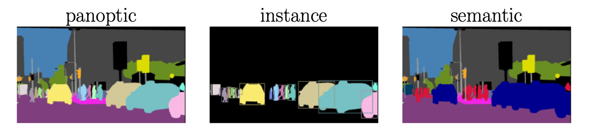
video instance segmentation (VIS),把实例分割出来
video semantic segmentation (VSS),只关心类别,不关心实例
video panoptic segmentation (VPS),实例和类别都关心
Open Vocabulary
在传统的计算机视觉任务中,通常会有一个固定的标签集合,即封闭词汇(Closed
Vocabulary)。然而,现实世界中的物体和场景是多样的,难以用一个固定的标签集合来描
述。为了应对这一挑战,研究者们提出了开放词汇(Open Vocabulary)的概念。
开放词汇指的是一种 可扩展的标签集合,它允许计算机视觉系统在遇到 新的物体或场
景 时,能够 自我更新 并学习到新的标签。这种方法可以让计算机视觉系统更好地适应现
实世界的多样性。
数据
开源数据
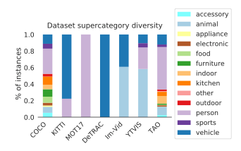
这是TAO论文中列举的一些数据集在类别占比方面的差异:
|---------------------------------------------------------------------------------------------------------------------------------------------------------------------------------------------------------------------------------------------------------|----------------------------------------------------------------------------------------------------------------------------------------------------------------------------------------------------------------------------------------------------------------------------------------------------------------------------------------------------------------------------------------------------------------------------------------------------------------------------------------------------------------------------------------------------------------------------------------------------------------------------------------------------------------------------------------------------------------------------------------------------------------------------------------------------------------------------------------------------------------------------------------------------------------------------------------------------------------------------------------------------------------------------------------------------------------------------------------------------------------------------------------------------------------------------------------------------------------------------------------------------------------------------------------------------------------------------------------------------------------------------------------------------------------------------------|
| 数据集名称 | 简介 |
| cocohttps://cocodataset.org/#home | COCO(Common Objects in Context)由微软团队于 2014 年创建,用于训练和评估 AI 模型。覆盖 80 种常见物体类别(如人、汽车、动物)和 91 种材料类别(如天空、墙壁) 对于分割任务,mask使用Run Length Encoding (RLE) scheme编码,提供API进行提取 分成3种标注,instances,stuff,panoptic。前面说的80类别是指instances,staff是草地,天空这种不可数,没有instance概念的。所以coco2017数据集有三个标注文件 captions_train2017.json描述的是每个image的license类型,ulr,宽度长度,id,拍摄时间等信息 和图片是根据file_name对应的,而不是顺序 但其实instances_val2017.json也有这个信息,在介绍完images之后才是annotations,里面包含了segmentation,bbox,等信息, person_keypoints_val2017.json多出的信息是keypoints。COCO 的 keypoints 就是一个 x, y, 可见性 的三元组重复 17 次拼成的长列表 person_keypoints_val2017.json的images中的图片不一定有人,也不一定有keypoints信息,所以还是要以coco.getAnnIds结果为准  |
|
| Cityscapeshttps://www.cityscapes-dataset.com | 在 50 个城市的春季、夏季和秋季 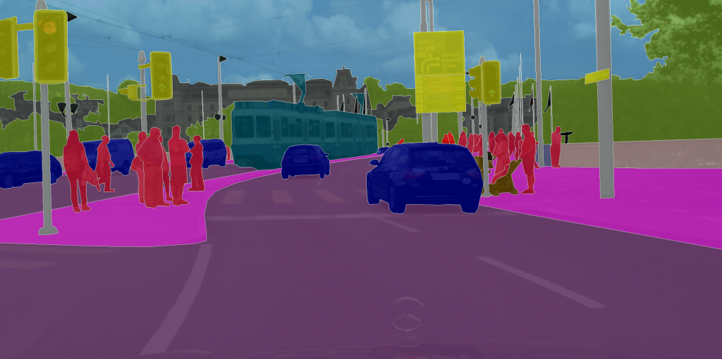 |
|
| YouTube-VOS Video Object Segmentation | 2019 version Training: 3471 videos, 65 categories and 6459 unique object instances. Validation: 507 videos, 65 training categories, 26 unseen categories and 1063 unique object instances. Test: 541 videos, 65 training categories, 29 unseen categories and 1092 unique object instances. 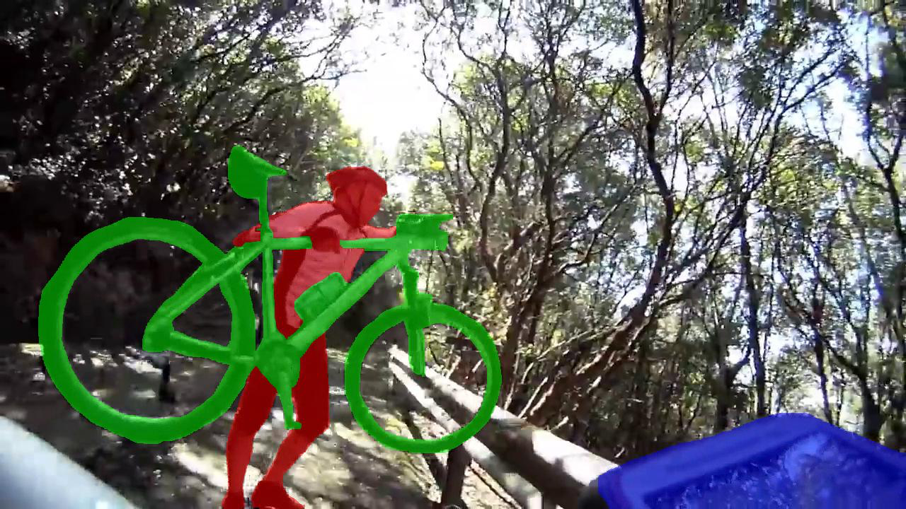 |
|
| LVIS (Large Vocabulary Instance Segmentation) https://github.com/FishYuLi/BalancedGroupSoftmax | Facebook AI Research (FAIR)针对针对长尾分布问题提出,所以看起来分得很细 使用COCO 2017的数据,只是标注是新的。每个图对应的标注能有80多个ann_ids ann_id因为全局唯一性,为了避免和COCO冲突,所以一般从5000开始编号 标注采用和COCO一样的方法,mask以多边形(Polygon) 保存在json中,使用lvis-api解码得到mask (pronounced 'el-vis') 1203 个类别中,有些只有几十个样本(如 "snowmobile"),而 "person" 有几十万个。person的类别id是793,这是WordNet synset 字典序排序得到的,不同于coco中person的类别id是1 除了person,还有person skiing,person riding a bike等类别,互斥关系 每个类别在json中都统计了出现image和instnce的次数,还有同义词等: "categories": { "image_count": 8, "synonyms": \[ "aerosol_can", "spray_can" , "def": "a dispenser that holds a substance under pressure", "id": 1, "synset": "aerosol.n.02", "name": "aerosol_can", "frequency": "c", "instance_count": 11 }, lvis_v1_val.json :"categories" 字段通常出现在 文件开头 lvis_v1_train.json :"categories" 字段出现在 文件末尾(在庞大的 "annotations" 数组之后) lvis = LVIS(json_path) all_cats=lvis.cats 可以得到所有类别 每个类别有frequency属性,分为f,c,r三类,表示frequent,common,rare,出现image的频率 https://docs.ultralytics.com/datasets/detect/lvis/ https://www.lvisdataset.org/dataset 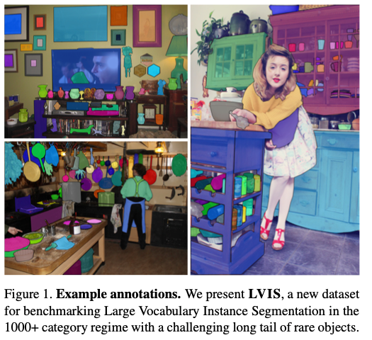 https://www.lvisdataset.org |
| TAO( Tracking Any Object) https://github.com/TAO-Dataset/tao/tree/master | 在multi-object tracking中对标COCO, 2,907段半分钟的视频,833 categories, https://taodataset.org/?spm=5176.28103460.0.0.18417551Y6B1Xl 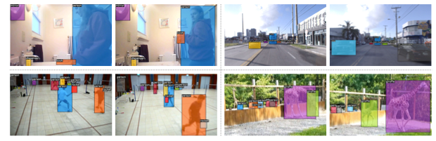 |
|
| MOT(multi object tracking) https://motchallenge.net/data/MOT17/ | 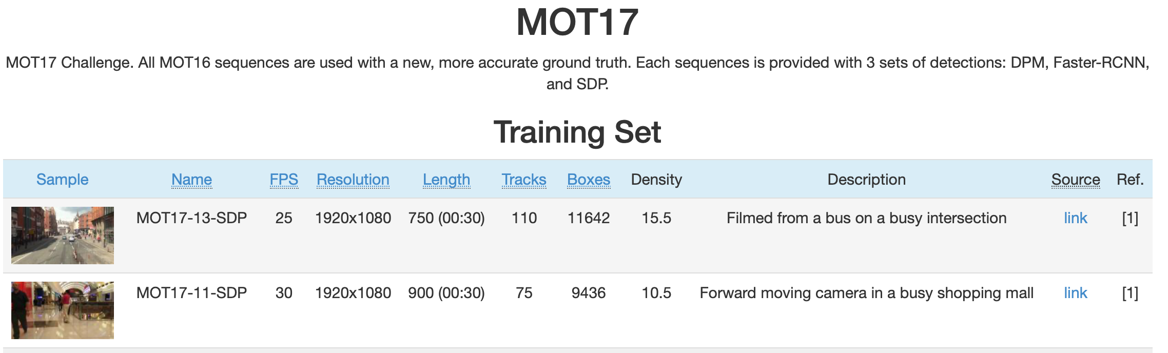 |
|
| DAVIS(Densely Annotated VIdeo Segmentation) https://davischallenge.org/?spm=5176.28103460.0.0.18417551Y6B1Xl | 无类别,只需要区分前景背景,使用mmsegmention,mask 时序传播 提供现成的mask图,不同instance以颜色区分,可以直接根据文件夹名字找到对应的类别/场景 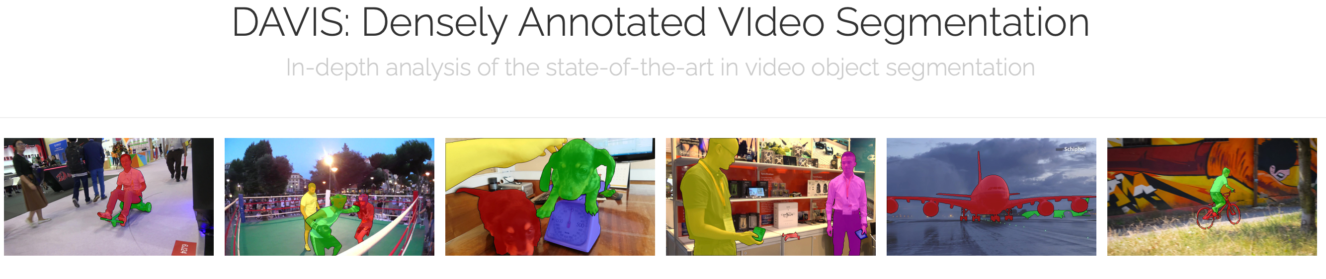 |
|
| MPII Human Pose Dataset | 图片有12.9G,标注是mat格式 https://www.mpi-inf.mpg.de/departments/computer-vision-and-machine-learning/software-and-datasets/mpii-human-pose-dataset/download |
生成/标注工具
MoMask https://github.com/EricGuo5513/momask-codes
WorldDreamer https://world-dreamer.github.io
Qwen-Image-Layered https://github.com/QwenLM/Qwen-Image-Layered/tree/main
使用了VAE把RGB和RGBA统一起来;使用Layer3D RoPE嵌入了layer索引信息;渐进学习,From Text-to-RGB to Text-to-RGBA,Text-to-RGBA to Text-to-Multi-RGBA,Text-to-Multi-RGBA to Image-to-Multi-RGBA
Grounded SAM https://github.com/IDEA-Research/Grounded-Segment-Anything
Sapiens https://github.com/facebookresearch/sapiens?tab=readme-ov-file
X-AnyLabeling https://github.com/CVHub520/X-AnyLabeling支持多种任务,典型的 C/S (Client/Server) 架构 设计,服务器端集成了各种模型,而客户端可以是多个并行标注。https://github.com/CVHub520/X-AnyLabeling/blob/main/docs/en/model_zoo.md
dataset/X-anylabel/X-AnyLabeling-Server/configs/models.yaml 没有被注视掉的就是要使用的模型
sam2.1_hiera_base_plus.pt,
-
- SAM 2.1 版本。
- 它是 SAM 2 的升级版(2024年底/2025年初发布),主要改进了小物体检测精度 、复杂场景下的分割稳定性 以及视频跟踪的长时记忆能力。相比 SAM 2,它修复了很多边缘情况的 Bug。
hiera:- 代表骨干网络架构使用的是 HiViT (Hierarchical Vision Transformer)。
图像分割算法
maskRCNN
https://wiki.math.uwaterloo.ca/statwiki/index.php?title=Mask_RCNN
2018年的文章,也是来自facebook FAIR团队,第一作者hekaiming。https://arxiv.org/pdf/1703.06870
在faster-RCNN基础上新增mask分支。
|-------------|----------------------------------------------------------------------------------------------------------------|----------------------------------------------------------------------------|
| | | |
| RCNN | 1.选择性搜索(Selective Search)得到2k个目标的候选区域 2.卷积神经网络(CNN)对每个区域进行特征提取 3. SVM做分类+regression回归得到bounding box | 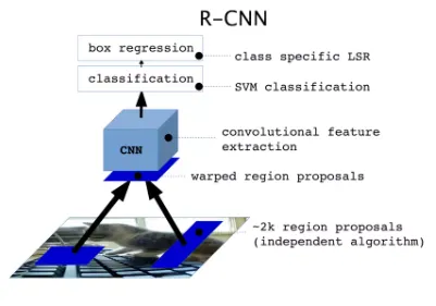 |
|
| Fast-RCNN | 1.选择性搜索(Selective Search)得到2k个目标的候选区域 2.卷积神经网络(CNN)对整个图进行特征提取再取候选区域 3. 特征图ROI Pooling共享池化,支持不同大小 4.FC同时完成分类和回归 | 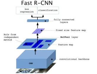 |
|
| Faster-RCNN | 把Fast-RCNN的第一步改成使用区域提议网络(RPN)生成区域提议 | 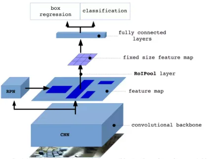 |
|
| Mask-RCNN | 在Faster-RCNN最后,增加一个mask branch用于分割 | 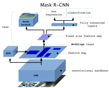 |
|
DETR
开启了transforme的时代
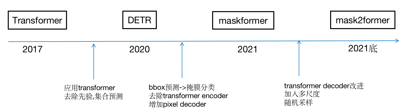
2020年的文章End-to-End Object Detection with Transformershttps://arxiv.org/pdf/2005.12872
https://github.com/facebookresearch/detr
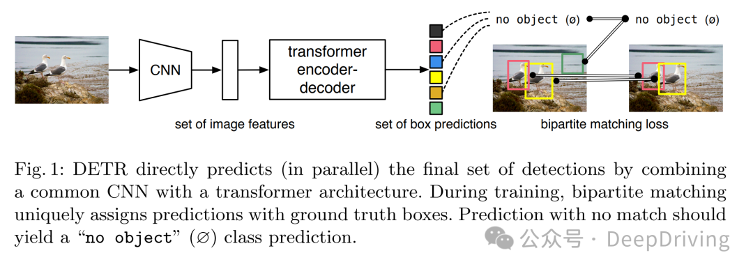
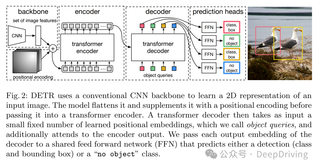
不需要anchor,不需要非极大值抑制( NMS)。第一个使用transformer到2D检测中。直接二分匹配box。CNN提取的特征和位置编码一起被送入encoder,然后是decoder,FFN:
Maskformer
2021年的文章,Per-Pixel Classification is Not All You Need for Semantic Segmentation
https://github.com/facebookresearch/MaskFormer
maskformer的基本思想是把语义分割、实例分割用一个统一的框架、损失和训练过程来实现。
Our key insight: mask classification is sufficiently general to solve
both semantic- and instance-level segmentation tasks in a unified manner using
the exact same model, loss, and training procedure.
以往都认为分割就是对每个像素做分类,但是这篇文章就告诉我们没必要这样:MaskFormer: Per-Pixel Classification is Not All You Need for Semantic Segmentation,直接预测一系列的二值mask。
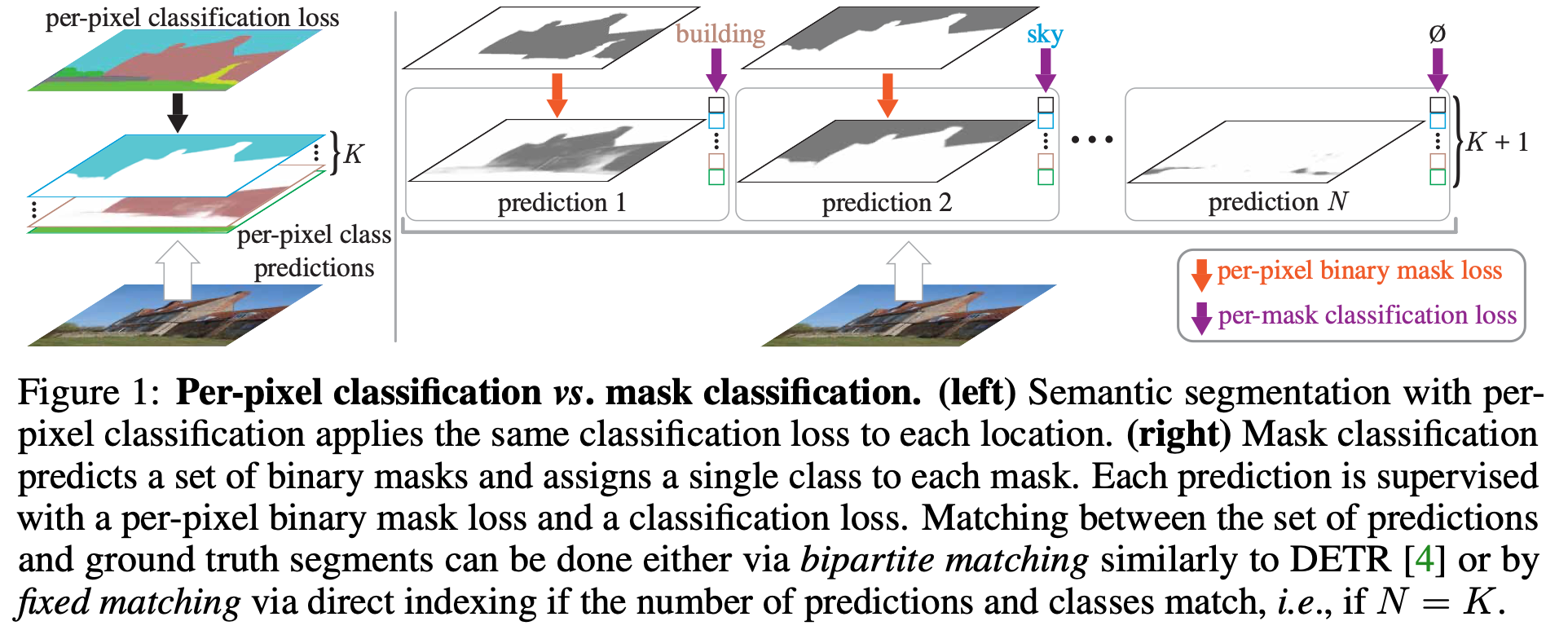
per-pixel的方法,每个pixel的位置使用相同的分类loss,而mask的方法,每个mask都有自己的per-pixel loss和per-mask loss。
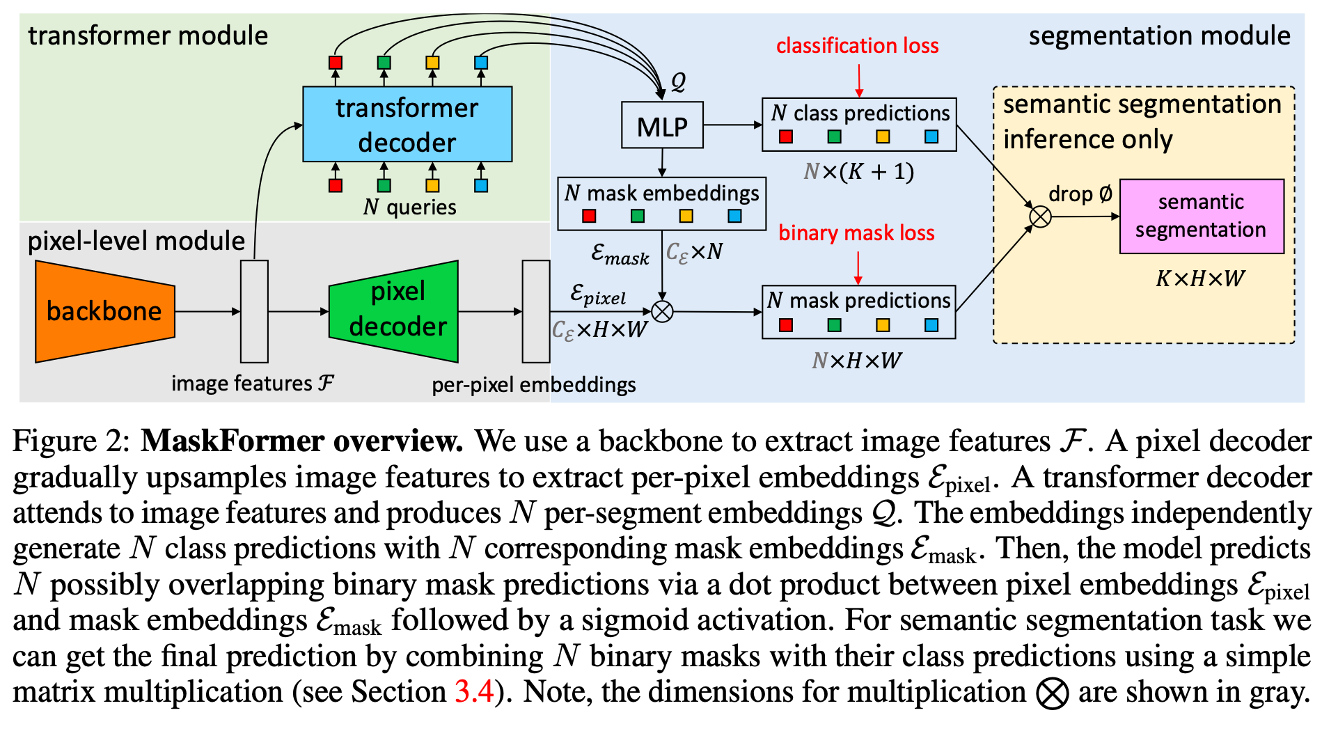
经过backbone之后,分别进行pixel decoder和transformer decoder,分别得到像素级别和mask级别的embeddings。因为要基于mask,所以mask embedding和pixel embedding结合得到binary mask loss。
Mask2Former
CVPR 2022
https://github.com/facebookresearch/Mask2Former
在Mask Transformer的基础上,又引入了Masked-attention,把cross-attention限制在预测的mask周围,所以叫mask2former。
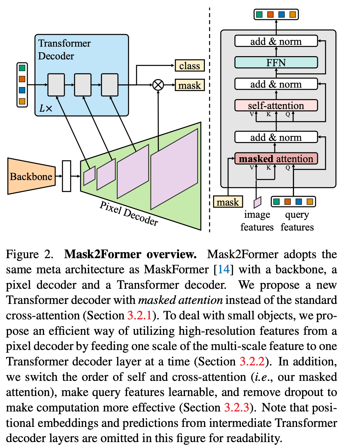
结构上和maskForme差不多,都是两个decoder,不过对transformer decoder进行了修改:增加了mask,并且交换了self attention和cross attention的位置,并且考虑到小物体,所以把每层的pxiel decoder送入了不同层的transformer decoder中。
SAM
https://github.com/facebookresearch/segment-anything
这是fecebook中更有名的分割算法,作者中仍然可以看到之前maskformer,DETR,mask2former的作者Alexander Kirillov。SAM其实是构建了分割的一整个系统,通过语言或者其他的prompt来指导模型去分割得到mask:
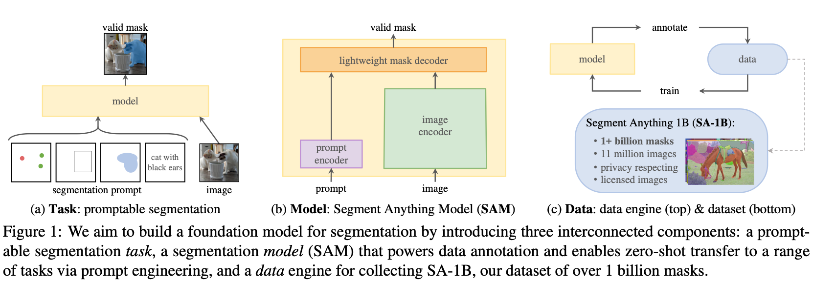
这些prompts可能是mask,points,box,text:
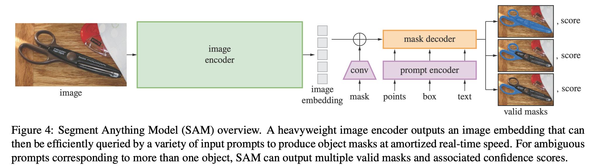
heavy的encoder得到embedding之后,利用这些prompt会得到对应的mask。参考代码:dataset/Ground-SAM/segment-anything/notebooks/automatic_mask_generator_example.ipynb
masks = mask_generator.generate(image)这里得到的masks是多个mask构成的list。每个mask除了mask本身外,还有area,bbox,predicted_iou等信息,在dataset/Ground-SAM/segment-anything/scripts/amg.py 中会把每个mask都保存下来,并且把这些属性保存在csv文件中。
python scripts/amg.py --checkpoint /home/zcg2/workspace/segmention/dataset/Ground-SAM/segment-anything/sam_vit_h_4b8939.pth --model-type vit_h --input /home/zcg2/workspace/segmention/dataset/Ground-SAM/segment-anything/notebooks/images/dog.jpg --output ./outSapiens
也是meta的,一次性可以完成四个任务;2D pose, part segmentation, depth, normal。也使用了OpenMMLab。
BiRefNet
Bilateral Reference for High-Resolution Dichotomous Image Segmentation
https://github.com/ZhengPeng7/BiRefNetCAAI AIR 2024
阿里联合南开等高校开发的用于高分辨率二分图像分割dichotomous image segmentation (DIS)。分为两个部分:
localization module (LM) and the reconstruction module (RM)
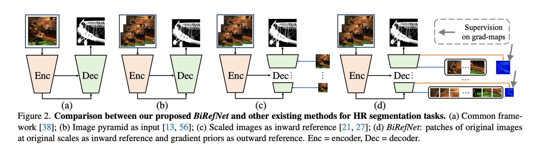
最左边是经典的Unet结构,b是把图像金字塔作为输入,c在b的基础上在decoder阶段也使用多尺度的图像。BIRefNet在c的基础上,使用的仍然是原始scale的原图,只不过切分成了patch(利用from einops import rearrange),并且使用了gradient priors(由拉普里斯得到)。
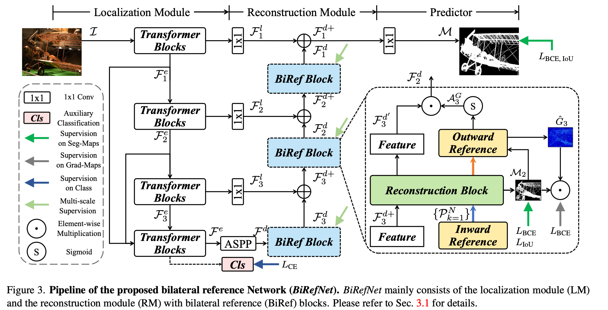
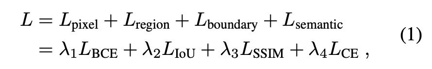
使用四种loss从四个方面去约束:
modenet
https://github.com/ZHKKKe/MODNet?tab=readme-ov-file#data-preparation
MODNet: Real-Time Trimap-Free Portrait Matting via Objective Decomposition (AAAI 2022)
matting objective decomposition network ,之前的要不是需要额外输入,要不是多阶段的,MODnet是第三种,分了两个并行的分支,分别是高分辨率和低分辨率的,分别提取边缘和主体(大致范围主要靠e-ASPP找到)。
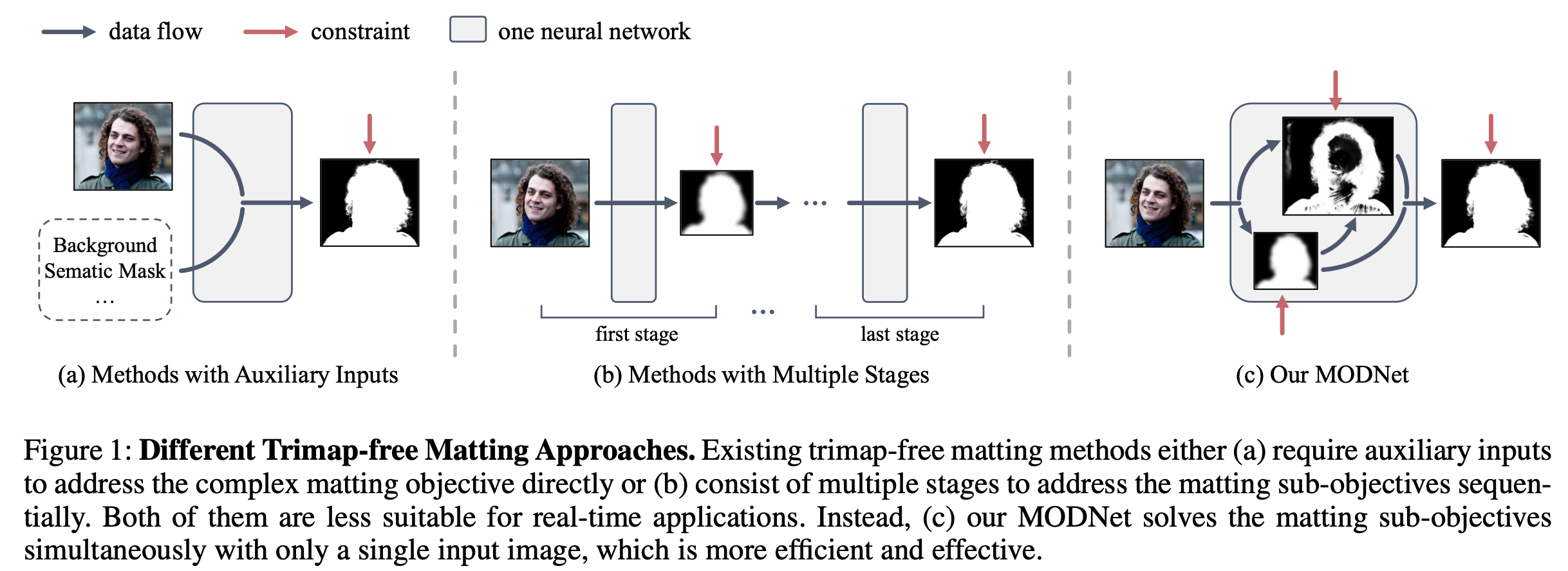
再加上最后的融合,所以MODNet 有三个branch,S(Semantic), D(detail), and F(fusion),计算三个输出s,d,alpha与真实值(Ground Truth)之间的误差,总损失函数是三部分之和。也可以看作是内部的"语义分支"自我生成一个隐式的 Trimap 指引,从而实现端到端的自动抠图。
S分支只需要提取高层特征,所以任何CNN结构都可以,这里选择的是MobileNetV2,最后一层sigmoid之后通道数为1。对应GT需要下采样16倍。为了解决空洞的问题,需要使用ASPP(Atrous Spatial Pyramid Pooling),但是ASPP计算量大,又使用了改进的e-ASPP,把参数量和计算量减小到了1%。ASPP核心是ASPP通过**并行使用不同膨胀率的空洞卷积,**e-ASPP则把空洞卷积也变成分离卷积,并且提前使用1x1解决降低了通道数。因为需要平滑一点,所以使用L2 loss。
D分支同时使用了原始图像I,还有S分支的最终特征还有S分支的低层特征。与S相比,D使用更少的卷积(12层),卷积的通道数也更少(最大通道数是64),并且为了减少计算量,也没一直保持原始的分辨率:在第一层就降低分辨率为1/4,在最后两层才恢复原来的分辨率。因为有skip link,所以donwsample的影响可以忽略不计。这个分支使用L1 loss,并且为了让它学习边缘,所以通过膨胀腐蚀得到mask去加权L1 loss。
F分支是CNN,把S输出上采样后和D的输出concatenate,然后得到最终的alpha输出。loss是L1 loss和compositional loss 的和。
因为制作GT成本很高,所以数据集都很小。普遍的做法是背景替换,但有泛化性的问题。观察到在训练集中不同分支间一致性比较高,在真实数据中一致性低,所以提出sub-objectives consistency (SOC),自监督地提高了在真实数据中的泛化性,本质是增强了三个输出之间的一致性,alpha分别和s和d计算L2和L1损失。问题是s缺失细节,容易把alpha也带偏,所以计算SOC时需要固定模型参数M,把SOC前后的M和M'的d和d'的L1 loss作为正则项。
训练中使用了合成数据,由前景和背景进行合成的数据集,类似论文 Deep Image Matting 里使用的数据集Composition-1k。PPM100数据集
PaddleSeg
需要安装paddle,千问说很多在线抠图工具的后端就是用的这个。对比MODNet, PP-MattingV2推理速度提升44.6%, 误差平均相对减小17.91%。
paddle可能对cuda支持不好,这时候sigmoid失效,导致出来的alpha有4条纹,所以可以直接用cpu推理:export CUDA_VISIBLE_DEVICES=""
https://github.com/JSHZT/ppmattingv2_pytorch/blob/main/Matting/docs/quick_start_en.md
https://github.com/PaddlePaddle/PaddleSeg
Deep Image Matting
https://sites.google.com/view/deepimagematting
MGMatting
Mask Guided Matting via Progressive Refinement Network
https://github.com/yucornetto/MGMatting
P3M-Net
https://github.com/ViTAE-Transformer/p3m-net
https://arxiv.org/pdf/2203.16828
没有使用到trimap,即便是HYBRID模式,分了两次推理,也只是img尺寸不一样,第一次得到的概率图用于第二次的后处理,而不是作为trimap送入网络中。
视频分割算法
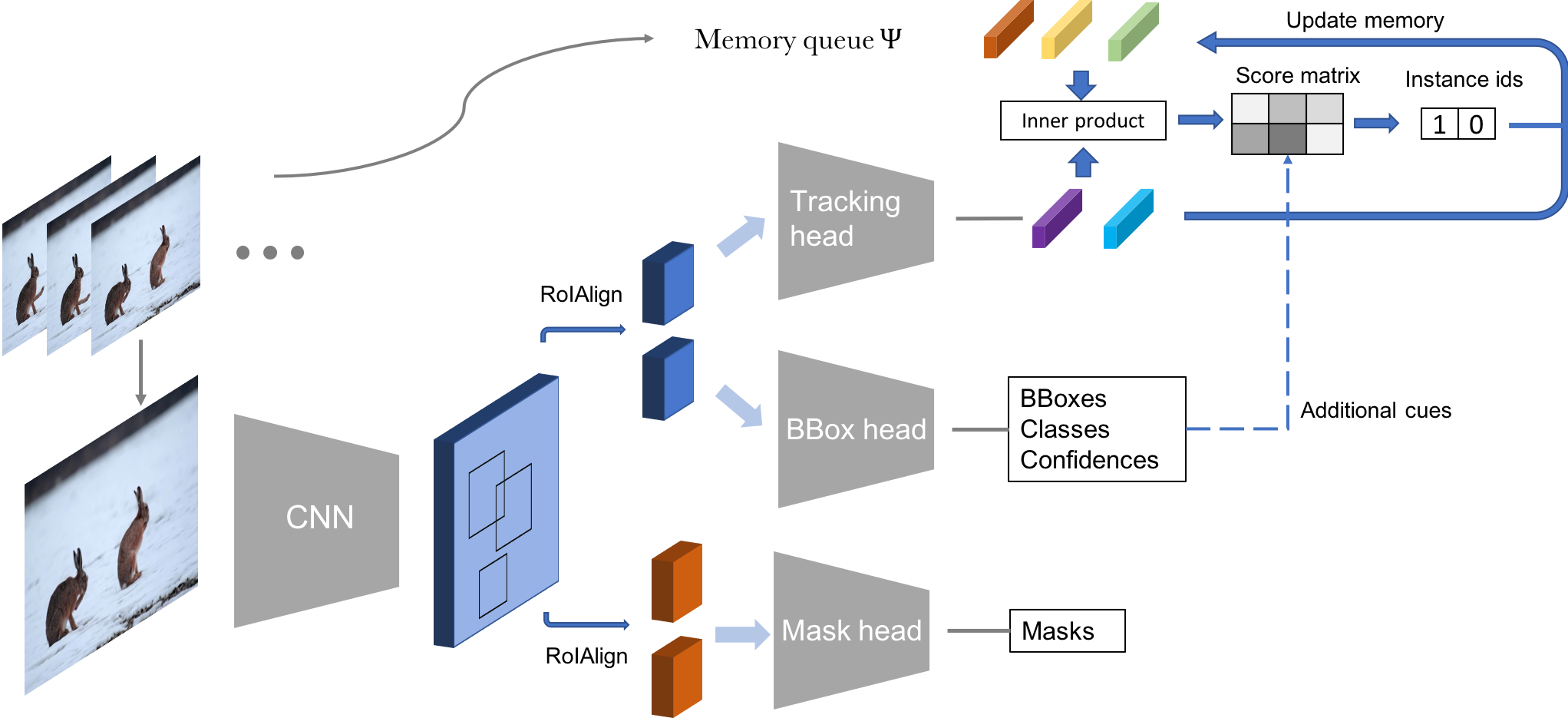
MaskTrackRCNN
2019年的文章,第一个提出来做视频实例分割,所以文章名字就叫Video Instance Segmentation。
https://github.com/youtubevos/MaskTrackRCNN
在maskRCNN基础上,又新加了racking branch,可以detect, segment, and track object instances,构建了YouTube-VIS数据集。
通过计算当前实例的特征与之前的实例的特征,可以得到当前实例属于之前出现过的N种内的哪个类别,或者是新出现的类别:
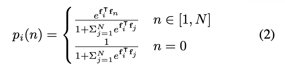
d
需要安装mmdetection (OpenMMLab 的目标检测工具箱):
git clone https://github.com/open-mmlab/mmdetection.git
cd mmdetection
pip install -r requirements/build.txt # 安装编译依赖
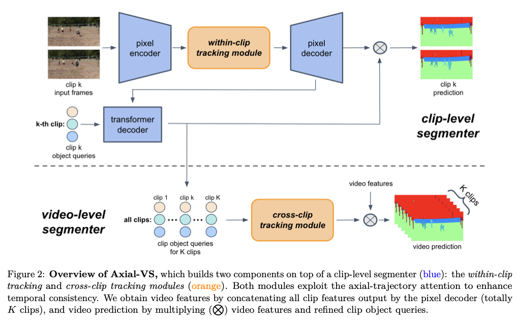
pip install -v -e . # 开发模式安装MaXTron
OpenAI等团队提出的视频分割技术https://github.com/TACJu/Axial-VS
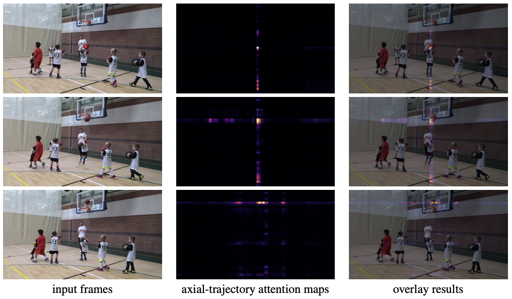
Clip-level的,一个clip就是由2~3帧组成的短视频。
DVIS+
https://github.com/KlingTeam/DVIS_Plus
D是decoupling,解藕成三部分:segmentation(使用Mask2Former), Referring Tracker, and Temporal Refiner
和CLIP结合后,又有了OV-DVIS++
需要安装detectron2,Detectron2是Facebook AI Research的检测和分割框架,其主要基于PyTorch实现,但具有更模块化设计,因此它是灵活且便于扩展的
python -m pip install 'git+https://gitcode.com/GitHub_Trending/de/detectron2.git'
python -m pip  install timm   # timm 是一个由 Ross Wightman 开发的 PyTorch 库,它提供了许多现代的图像分类模型,旨在加速研究和开发
PP-HumanSeg(百度), 目前工业界在手机端人像分割的标杆
**MediaPipe Segmentation (Google),**Zoom/Google Meet 里看到的背景虚化技术,使用了图结构搜索 (NAS) 找到的最优架构
CIRKD
modnet
DiffusinMat
matteformer
Label_Assisted_Distillation-main
u2net
mmdetction
loss
- Dice loss
就是计算交并比
def _DiceLoss(self, pred, gt): # [N, C, H, W] one-hot
        gt_fore = gt[:,1,:,:]
        pred_fore = pred[:,1,:,:]
        intersection = (pred_fore * gt_fore).sum()
        pred_fore = pred_fore.contiguous().view(-1)
        gt_fore = gt_fore.contiguous().view(-1)
        dice_coeff = (2. * intersection + 1e-5) / (pred_fore.sum() + gt_fore.sum() + 1e-5)

return 1 - dice_coeff- 交叉熵
看作分类,当然可以使用交叉熵
def _loss(self, true, pred):
        pred = torch.maximum(torch.minimum(pred, torch.tensor(1 - 1e-15, dtype=torch.float32)), torch.tensor(1e-15, dtype=torch.float32))
        softmax_loss = -torch.sum(true * torch.log(pred), dim=1) # [N, C, H, W] -> [N, H, W]
return softmax_loss # true是二通道的one-hot编码,pred是softmax的输出- 编译BCE
对图像分割边缘计算BCE,nn.BCELoss(reduction='mean') 是 PyTorch 中专门用于二分类任务(或每个像素做二分类的语义分割任务)的损失函数。reduction='mean' 表示它会自动计算并返回当前批次(batch)中所有元素损失的平均值。
BCELoss 内部会计算对数(log),它假设传入的 pred 已经经过了 Sigmoid 激活函数。如果你的网络最后一层输出的是原始分数(Logits,即没有经过 Sigmoid),请直接改用 nn.BCEWithLogitsLoss。它不仅用法一样,而且在数值计算上更加稳定。
import torch
import torch.nn as nn
import torch.nn.functional as F

class YourModel(nn.Module):
    def __init__(self):
        super().__init__()
        # 初始化 BCELoss,reduction='mean' 是默认值,表示对 batch 内所有元素求平均
        self.bce = nn.BCELoss(reduction='mean')

    def _boundaryBCE_loss(self, pred, gt):
        # 1. 提取前景通道,保持在 GPU/CPU 上,不要转 numpy!
        # 使用 .detach() 是因为在生成边界 mask 时不需要梯度,避免 inplace 操作报错
        pred_fore = pred[:, 1, :, :].detach()
        gt_fore = gt[:, 1, :, :].detach()

        # 2. 二值化 (使用 PyTorch 原生操作)
        binary_pred = (pred_fore > 0.5).float()
        binary_gt = (gt_fore > 0).float()

        # 3. 模拟膨胀和腐蚀 (使用 PyTorch 的 max_pool2d 和 avg_pool2d)
        # 注意:pooling 需要 [N, 1, H, W] 的输入,所以要 unsqueeze(1)
        kernel_size = 8
        # 最大池化 = 膨胀 (Dilation)
        dilation_gt = F.max_pool2d(binary_gt.unsqueeze(1), kernel_size=kernel_size, stride=1, padding=kernel_size//2).squeeze(1)
        # 最小池化 = 腐蚀 (Erosion)
        # PyTorch 没有直接的 min_pool,可以用 -max_pool(-x) 来巧妙实现
        erode_pred = -F.max_pool2d(-binary_pred.unsqueeze(1), kernel_size=kernel_size, stride=1, padding=kernel_size//2).squeeze(1)
        erode_gt = -F.max_pool2d(-binary_gt.unsqueeze(1), kernel_size=kernel_size, stride=1, padding=kernel_size//2).squeeze(1)

        # 4. 提取边界宽度
        boundary_width_pred = (pred_fore - erode_pred)
        boundary_width_pred = (boundary_width_pred > 0).float()

        boundary_width_gt = (dilation_gt - erode_gt)
        boundary_width_gt = (boundary_width_gt > 0).float()

        # 5. 生成边界区域的预测和真值
        pred_boundary = boundary_width_pred * pred_fore
        gt_boundary = boundary_width_gt * gt_fore

        # 6. 计算 BCE 损失 (传入的必须是 float 类型的 Tensor)
        boundaryBCE_loss = self.bce(pred_boundary, gt_boundary)

return boundaryBCE_lossreference:
1.https://developer.volcengine.com/articles/7403569858836856843