最近刷到了「图绘科研」作者为 QDY 的原创教程《图绘科研|MATLAB科研绘图:土地利用转移桑基图绘制教程》,突然意识到我之前开发的桑基图绘图工具,要画这类图像的话,要生成全局邻接矩阵会有点麻烦,因此专门写了个全局邻接矩阵生成函数 mergeAdjMat 来实现这个功能,本文涉及到的桑基图绘制工具及邻接矩阵生成函数可在以下任意仓库获取 (因为该工具我一直在维护,在仓库能用到最新版,所以最好还是去仓库下载,本文提到的四个例子请见仓库内的 例0、例16-例18):
- 【gitee】https://gitee.com/slandarer/matlab-sankey-diagram
- 【github】https://github.com/slandarer/MATLAB-sankey-plot
- 【fileexchange】https://ww2.mathworks.cn/matlabcentral/fileexchange/128679-sankey-plot
封面图:
基础使用
例如我们有四层,每两层之间有一邻接矩阵,我们可以使用 mergeAdjMat 函数构造全局邻接矩阵来画图,代码非常短:
matlab
% Define inter-layer adjacency matrices
% 定义层间邻接矩阵
A12 = [1,2,1; 1,2,3; 2,0,1];
A23 = [1,4; 2,1; 0,3];
A34 = [1,5; 2,3];

% Assemble global block matrix (main diagonal = O, super-diagonal = A12, A23, A34)
% 组装全局分块矩阵 (主对角线为零矩阵,上对角线为 A12, A23, A34)
adjMat = mergeAdjMat({A12, A23, A34});

SK = SSankey([],[],[], 'AdjMat',adjMat);
SK.draw()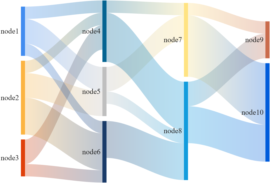
想要更改节点名称可以在绘图前设置 NodeList 属性:
matlab
SK = SSankey([],[],[], 'AdjMat',adjMat);
SK.NodeList = {'A','B','C','A','B','C','A','B','A','B'};
SK.draw()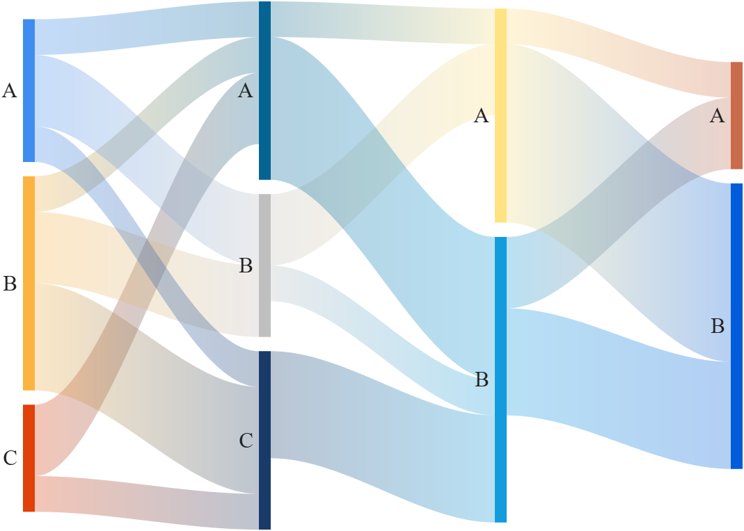
等价代码
以下两种代码等价:
使用节点-流量链接表 (links)
matlab
figure()
% Define links
links = {'a', 'A', 3; 'a', 'B', 1; 'a', 'C', 1;
        'b', 'A', 1; 'b', 'B', 5;
        'c', 'B', 2; 'c', 'C', 4;
        'A', 'AA', 4; 'A', 'CC', 1;
        'B', 'BB', 5; 'B', 'CC', 3;
        'C', 'AA', 5};

% 创建桑基图对象(Create a Sankey diagram object)
SK1 = SSankey(links(:,1), links(:,2), links(:,3));

% 设置节点顺序及层次(Set node order and layer)
SK1.NodeList = {'a', 'b', 'c', 'A', 'B', 'C', 'AA', 'BB', 'CC'};
SK1.Layer = [1, 1, 1, 2, 2, 2, 3, 3, 3];

% 开始绘图(Start drawing)
SK1.draw()
使用多个层间邻接矩阵 (adjMat)
matlab
figure()
% 定义层间邻接矩阵(Define inter-layer adjacency matrices)
A12 = [3,1,1; 1,5,0; 0,2,4];   % a,b,c -> A,B,C
A23 = [4,0,1; 0,5,3; 5,0,0];   % A,B,C -> AA,BB,CC

% 组装全局分块矩阵(Assemble global block matrix)
% 主对角线为零,上对角线为 A12, A23(main diagonal = zero, super-diagonal = A12, A23)
adjMat = mergeAdjMat({A12, A23});

SK2 = SSankey([], [], [], 'AdjMat',adjMat);

% 设置节点名称(Set node names)
SK2.NodeList = {'a', 'b', 'c', 'A', 'B', 'C', 'AA', 'BB', 'CC'};

SK2.draw()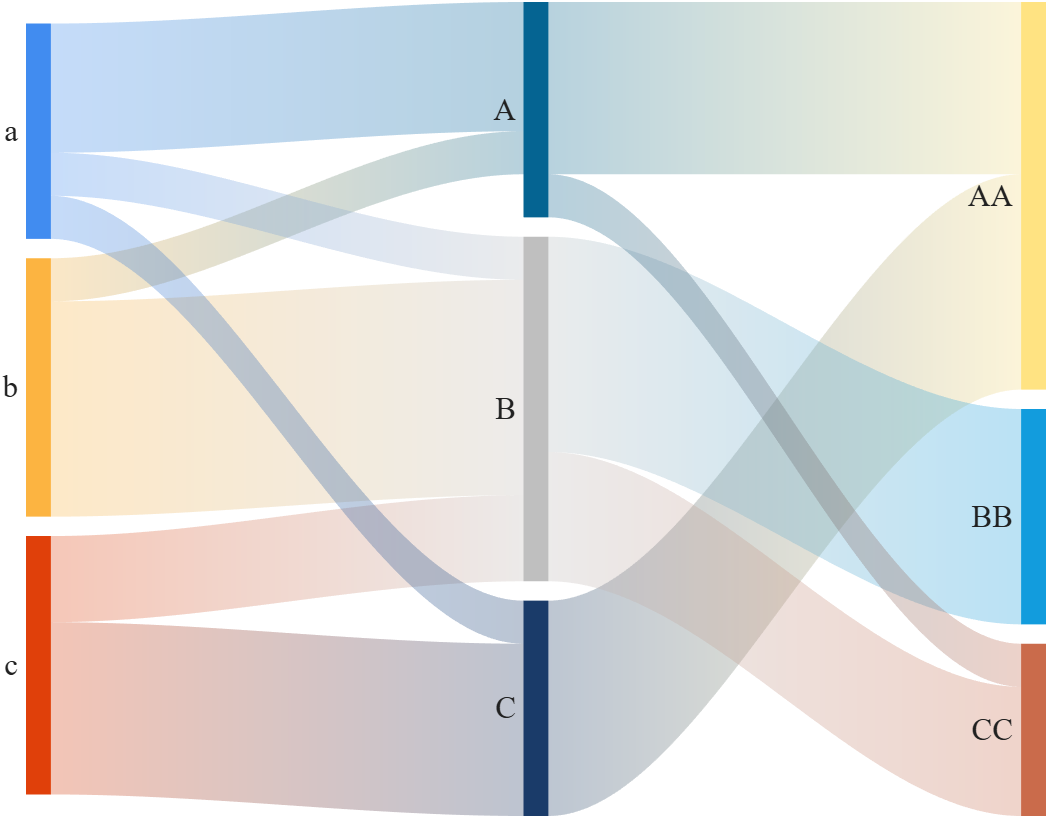
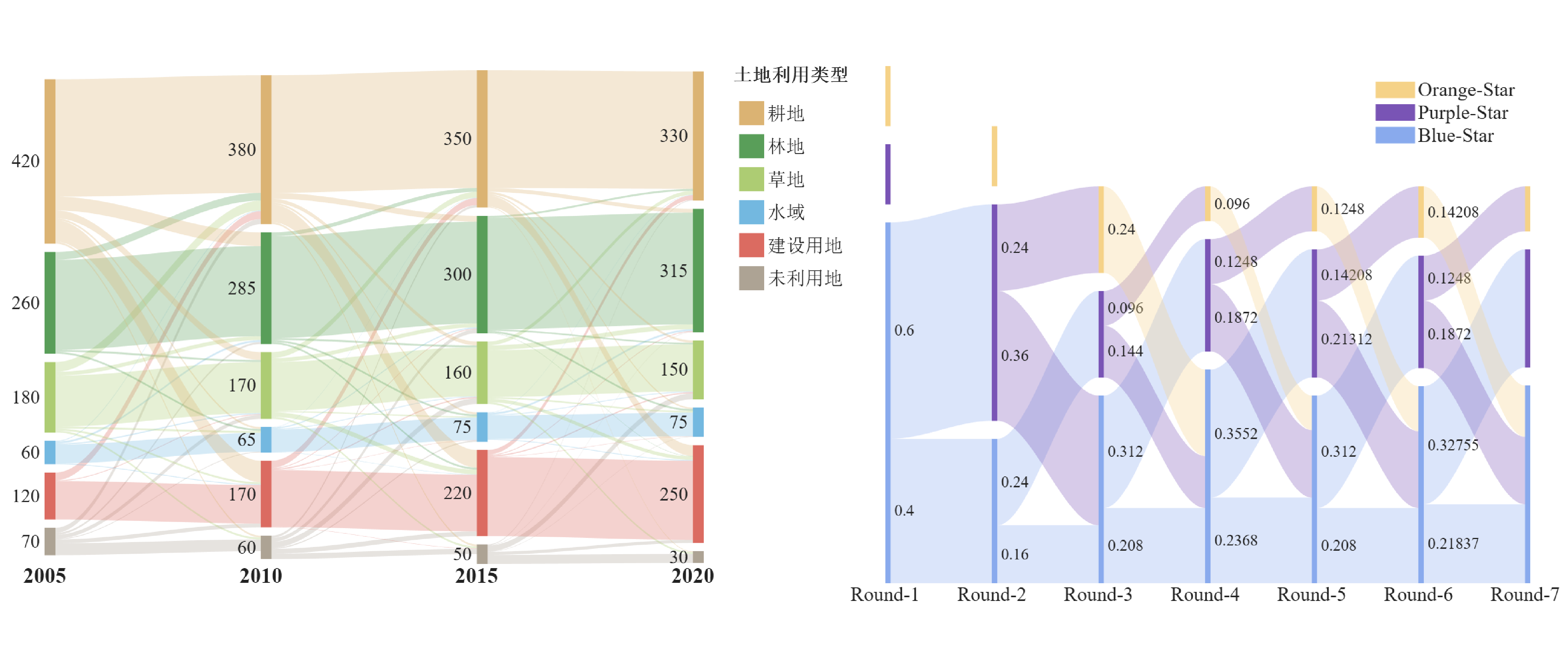
土地利用变化桑基图
注释写的还是比较清楚的,这里我是算了一下节点流量来当作节点标签:
matlab
% 本示例来源于微信公众号「图绘科研」的原创教程
% 《图绘科研|MATLAB科研绘图:土地利用转移桑基图绘制教程》,作者为 QDY

figure('Name','sankey demo17', 'Units','normalized', 'Position',[.05,.2,.6,.6])

layerNames = {'2005', '2010', '2015', '2020'};
nodeNames  = {'耕地', '林地', '草地', '水域', '建设用地', '未利用地'};
LN = length(layerNames); NN = length(nodeNames);

nodeTitle  = '土地利用类型';
CList = [.86, .70, .45;   % 耕地:浅棕色
         .35, .62, .35;   % 林地:绿色
         .68, .80, .45;   % 草地:黄绿色
         .45, .72, .88;   % 水域:蓝色
         .86, .42, .38;   % 建设用地:红橙色
         .68, .64, .58];  % 未利用地:灰褐色
T12 = [300,  35,  20,  5, 55,  5;
        20, 230,   5,  5,  0,  0;
        25,  10, 130,  5,  5,  5;
         2,   5,   3, 48,  2,  0;
        20,   0,   2,  0, 98,  0;
        13,   5,  10,  2, 10, 30];  % 2005 -> 2015
T23 = [300,  15,  10,  5,  45,  5;
        10, 260,   5,  5,   5,  0;
        15,  10, 125,  3,  12,  5;
         1,   3,   2, 58,   1,  0;
        18,   2,   3,  1, 145,  1;
         6,  10,  15,  3,  12, 14]; % 2015 -> 2020
T34 = [300,  10,   6,  4,  28,  2;
         5, 285,   4,  5,   1,  0;
        10,  12, 120,  4,   9,  5;
         1,   5,   2, 60,   2,  0;
        12,   2,   3,  1, 202,  0;
         2,   1,  15,  1,   8, 23]; % 2020 -> 2022

% 获取全局邻接矩阵 (Assemble global block matrix)
layerAdj = {T12, T23, T34};
adjMat = mergeAdjMat(layerAdj);

% 计算节点流量 (Compute node values)
nodeVal = zeros(NN, LN);
for i = 1:(LN - 1)
    nodeVal(:, i)     = max(nodeVal(:, i), sum(layerAdj{i}, 2));
    nodeVal(:, i + 1) = max(nodeVal(:, i + 1), sum(layerAdj{i}, 1).');
end

% 创建桑基图对象 (Create sankey plot object)
SK = SSankey([],[],[], 'AdjMat',adjMat);
SK.RenderingMethod = 'left';                 % 链接与左侧节点颜色相同 (Rendering Method : 'left')
SK.ColorList = repmat(CList, [LN, 1]);       % 为每个节点分配颜色 (Assign colors to all nodes)
SK.NodeList = cellstr(num2str(nodeVal(:)));  % 设置节点标签 (Set node labels)
% SK.NodeList = arrayfun(@(x) num2str(x), nodeVal(:), 'UniformOutput', false);
SK.LabelLocation = 'left';                   % 设置节点标签位于左侧 (Place labels on left side)
SK.draw()

% 添加层标签及图例 (Add layer labels and legend)
text(1:LN, zeros(1, LN), layerNames, ...
    'HorizontalAlignment','center', 'VerticalAlignment','top', ...
    'FontName','Times New Roman', 'FontSize',17, 'FontWeight','bold')
set(gca, 'Positio',[.13, .11, .68, .815]);
lgdHdl = legend(SK.BlockHdl(1:NN), nodeNames, ...
    'FontSize',15, 'Box','off', 'FontName','宋体');
lgdHdl.Title.String = nodeTitle;
lgdHdl.Position = [.8, .55, .2, .4];
lgdHdl.ItemTokenSize = [20, 20];
如果设置土地类型为 NodeList:
matlab
SK.NodeList = repmat(nodeNames, [1, LN]);
SK.LabelLocation = 'center';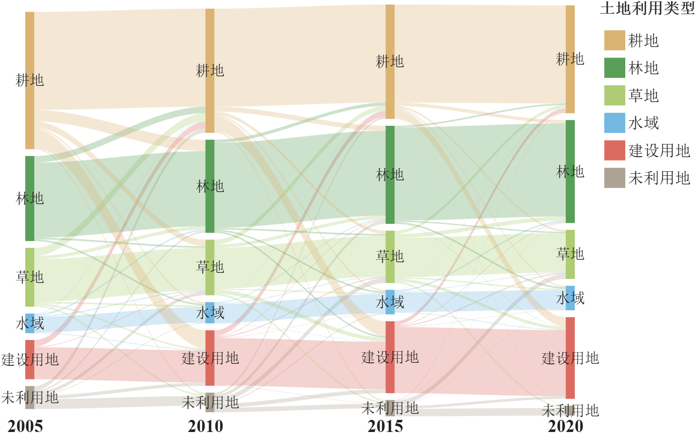
状态转移矩阵桑基图
状态转移矩阵可视化,以代号鸢黄月英唤星为例,初始状态全为蓝色(状态3),蓝色有60%概率变成紫色(状态2),有40%概率维持蓝色不变。紫色有60%概率跳回蓝色,有40%概率变成橙色,橙色(状态1)的下一状态一定是蓝色。
matlab
% 定义状态转移矩阵 (Define transition matrix S)
S = [0, .4, .0;
     0, .0, .6;
     1, .6, .4];
% 初始状态向量 (Initial state vector)
s0 = [0; 0; 1];
% 时间层数量 (Number of time layers)
LN = 7; NN = size(S, 1);
% 状态颜色配置 (Color palette for states)
CList = [245,210,136; 121, 84,181; 137,170,237]./255;

layerNames = compose('Round-%d', 1:LN);
nodeNames = {'Orange-Star', 'Purple-Star', 'Blue-Star'};

% 计算状态随时间分布 (Compute state distribution over time)
states = zeros(NN, LN - 1);
states(:,1) = s0;
for t = 2:(LN - 1)
    states(:, t) = S * states(:, t - 1);
end
% 构建层间邻接矩阵 (Build inter-layer adjacency matrices)
A = rot90(fliplr(S));
layerAdj = cell(1, LN - 1);
for t = 1:(LN - 1)
    layerAdj{t} = diag(states(:, t))*A;
end
% 绘制桑基图 (Render the Sankey diagram)
adjMat = mergeAdjMat(layerAdj);
SK = SSankey([],[],[], 'AdjMat',adjMat);
SK.Layer = kron(1:LN, ones(1, NN));
SK.ColorList = repmat(CList, [LN, 1]);
SK.NodeList = repmat({''}, 1, LN*NN);
SK.RenderingMethod = 'left';
SK.ValueLabelLocation = 'left';
SK.Align = 'down';
SK.draw()

legend(SK.BlockHdl(1:NN), nodeNames, 'FontSize',15, 'FontName','Times New Roman', 'Box','off')
ax = gca;
text(1:LN, ones(1, LN).*ax.YLim(2), layerNames, ...
    'HorizontalAlignment','center', 'VerticalAlignment','top', ...
    'FontName','Times New Roman', 'FontSize',15)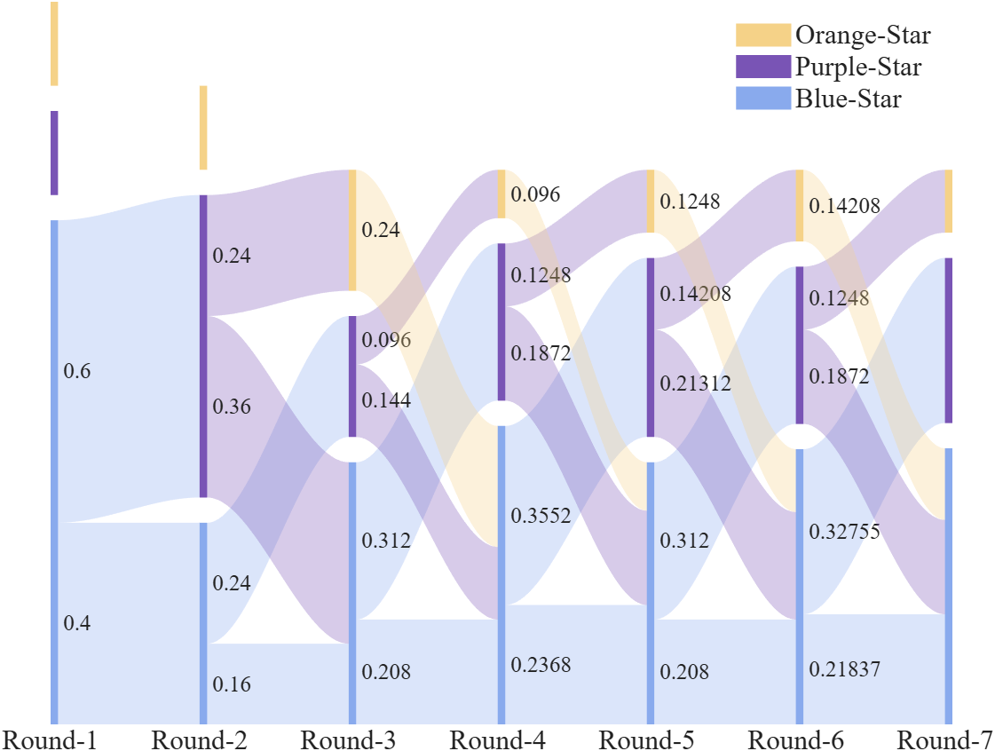
当然如果我们把 layer number (LN) 调大些,各种状态的比例会趋于稳定:
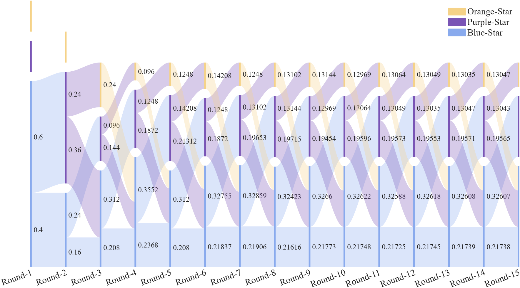
(像个蜈蚣。。。。)
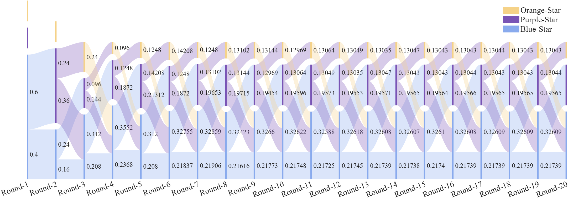
(更像了。。。。。)