论文地址:
https://www.sciencedirect.com/science/article/pii/S0008884625002467
论文题目:
A transfer learning-driven paradigm for understanding cryogenic freezing mechanisms in low water/binder cement-based composites
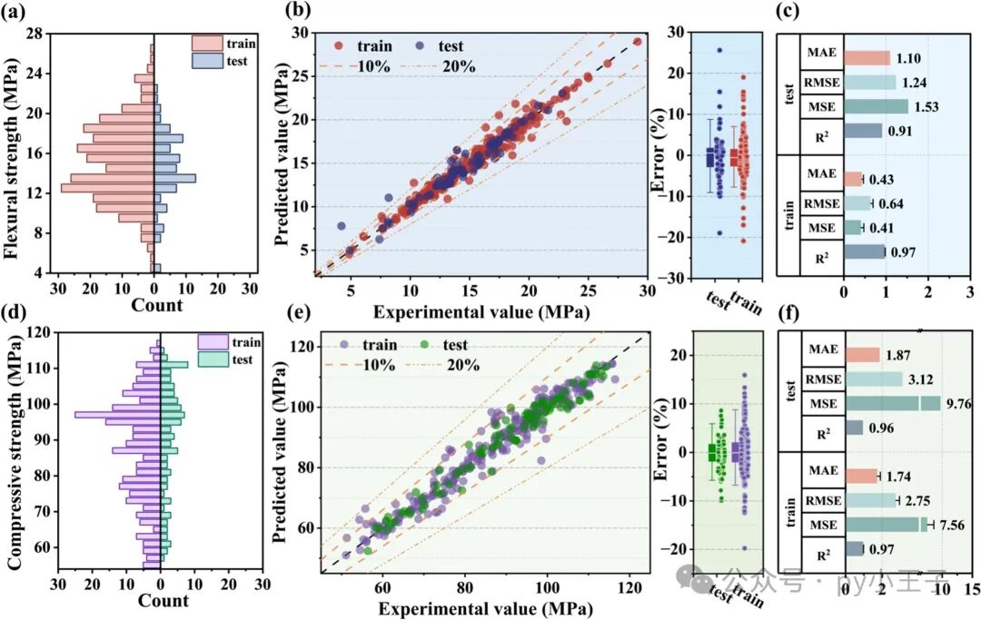
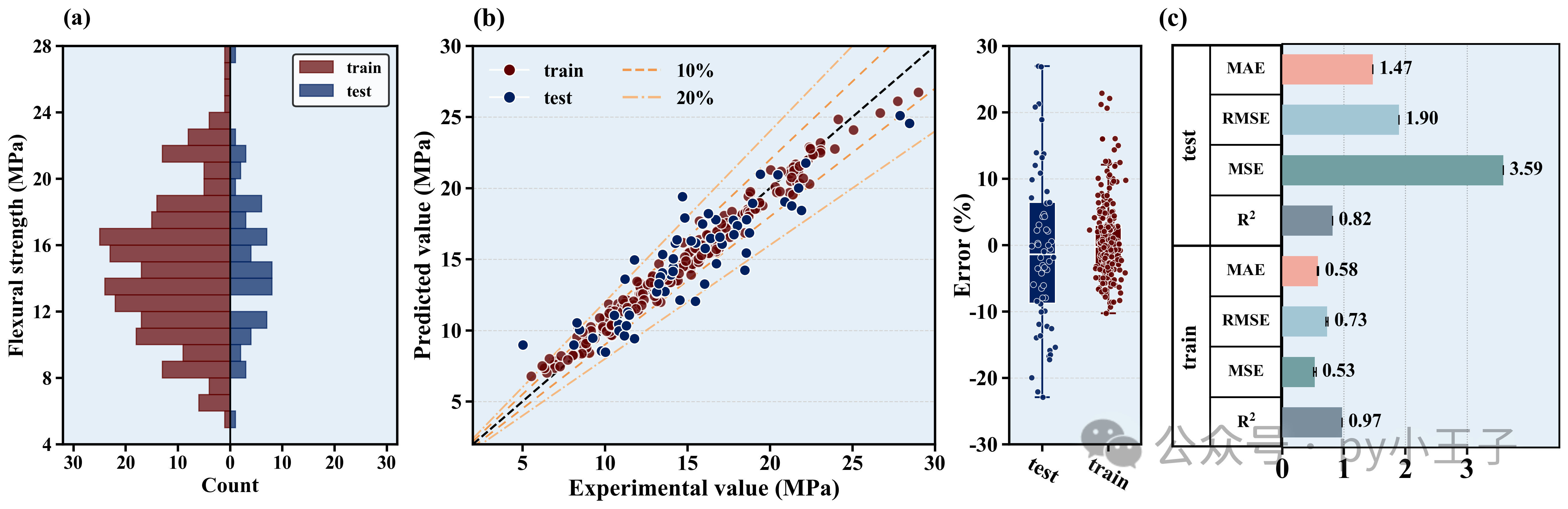
图 1 抗弯强度预测模型结果可视化综合图:该图展示随机森林回归模型对材料抗弯强度的预测效果及数据分布特征。(a) 子图为训练集与测试集抗弯强度双向直方图,左侧红色柱形代表训练集样本数量分布,右侧深蓝色柱形代表测试集样本数量分布,直观呈现数据集的样本分布特征;(b) 子图左侧为实验值与预测值的散点拟合图,横坐标为实验抗弯强度,纵坐标为模型预测抗弯强度,黑色虚线为理想拟合线,橙色与浅橙色虚线分别代表 ±10%、±20% 误差区间,红色散点为训练集、深蓝色散点为测试集,散点越贴近理想拟合线代表模型预测精度越高,右侧为训练集与测试集预测相对误差箱线图,清晰展示两组数据的误差分布范围;(c) 子图为模型训练集与测试集的 R²、MSE、RMSE、MAE 评价指标柱状图,直观对比模型在训练与预测阶段的性能表现。正式图注:图 1 随机森林模型抗弯强度预测结果的样本分布、拟合效果及性能评价综合可视化图。
复现图片:
配色方案:
python
COLOR_SCHEMES = {
    1: {'bg': '#e4eff7', 'train': '#610000', 'test': '#002060', 'line10': '#f0984d', 'line20': '#f5b881', 'r2': '#7a8e9e', 'mse': '#729fa1', 'rmse': '#a2c6d4', 'mae': '#f2aa9e'},
    2: {'bg': '#f9f2ec', 'train': '#d95f02', 'test': '#7570b3', 'line10': '#1b9e77', 'line20': '#66c2a5', 'r2': '#8da0cb', 'mse': '#e78ac3', 'rmse': '#a6d854', 'mae': '#ffd92f'},
    3: {'bg': '#f0f5f0', 'train': '#e41a1c', 'test': '#377eb8', 'line10': '#4daf4a', 'line20': '#98df8a', 'r2': '#9ebcda', 'mse': '#8c6bb1', 'rmse': '#88419d', 'mae': '#810f7c'},
    4: {'bg': '#f7f4f9', 'train': '#984ea3', 'test': '#ff7f00', 'line10': '#a65628', 'line20': '#e41a1c', 'r2': '#b3cde3', 'mse': '#ccebc5', 'rmse': '#decbe4', 'mae': '#fed9a6'},
    5: {'bg': '#f5f5f5', 'train': '#c51b7d', 'test': '#4d9221', 'line10': '#d01c8b', 'line20': '#f1b6da', 'r2': '#fbb4ae', 'mse': '#b3cde3', 'rmse': '#ccebc5', 'mae': '#decbe4'},
    6: {'bg': '#edf8fb', 'train': '#8c6bb1', 'test': '#88419d', 'line10': '#8c96c6', 'line20': '#bfd3e6', 'r2': '#1b9e77', 'mse': '#d95f02', 'rmse': '#7570b3', 'mae': '#e7298a'},
    7: {'bg': '#ffffcc', 'train': '#d73027', 'test': '#4575b4', 'line10': '#fc8d59', 'line20': '#fee090', 'r2': '#66c2a5', 'mse': '#fc8d62', 'rmse': '#8da0cb', 'mae': '#e78ac3'},
    8: {'bg': '#f0f9e8', 'train': '#0868ac', 'test': '#43a2ca', 'line10': '#7bccc4', 'line20': '#a8ddb5', 'r2': '#a6cee3', 'mse': '#1f78b4', 'rmse': '#b2df8a', 'mae': '#33a02c'},
    9: {'bg': '#fff5eb', 'train': '#7f2704', 'test': '#d94801', 'line10': '#f16913', 'line20': '#fd8d3c', 'r2': '#fb9a99', 'mse': '#e31a1c', 'rmse': '#fdbf6f', 'mae': '#ff7f00'},
    10: {'bg': '#fcfbfd', 'train': '#3f007d', 'test': '#6a51a3', 'line10': '#807dba', 'line20': '#bcbddc', 'r2': '#cab2d6', 'mse': '#6a3d9a', 'rmse': '#ffff99', 'mae': '#b15928'},
    11: {'bg': '#f5f0f0', 'train': '#67001f', 'test': '#053061', 'line10': '#d6604d', 'line20': '#4393c3', 'r2': '#8dd3c7', 'mse': '#ffffb3', 'rmse': '#bebada', 'mae': '#fb8072'},
    12: {'bg': '#eef5e5', 'train': '#00441b', 'test': '#40004b', 'line10': '#1b7837', 'line20': '#762a83', 'r2': '#80b1d3', 'mse': '#fdb462', 'rmse': '#b3de69', 'mae': '#fccde5'},
    13: {'bg': '#f7f7f7', 'train': '#252525', 'test': '#737373', 'line10': '#525252', 'line20': '#969696', 'r2': '#d9d9d9', 'mse': '#bdbdbd', 'rmse': '#969696', 'mae': '#737373'},
    14: {'bg': '#f0f4f5', 'train': '#b2182b', 'test': '#2166ac', 'line10': '#d6604d', 'line20': '#92c5de', 'r2': '#f4a582', 'mse': '#fddbc7', 'rmse': '#d1e5f0', 'mae': '#4393c3'},
    15: {'bg': '#faebd7', 'train': '#800000', 'test': '#000080', 'line10': '#cd5c5c', 'line20': '#f08080', 'r2': '#ffc0cb', 'mse': '#ffb6c1', 'rmse': '#ff69b4', 'mae': '#ff1493'},
    16: {'bg': '#f5fffa', 'train': '#2e8b57', 'test': '#8b0000', 'line10': '#3cb371', 'line20': '#cd5c5c', 'r2': '#00fa9a', 'mse': '#00ff7f', 'rmse': '#90ee90', 'mae': '#98fb98'},
    17: {'bg': '#ffebcd', 'train': '#8b4513', 'test': '#2f4f4f', 'line10': '#a0522d', 'line20': '#cd853f', 'r2': '#d2b48c', 'mse': '#f4a460', 'rmse': '#daa520', 'mae': '#b8860b'},
    18: {'bg': '#f0ffff', 'train': '#008b8b', 'test': '#9932cc', 'line10': '#20b2aa', 'line20': '#ba55d3', 'r2': '#e0ffff', 'mse': '#afeeee', 'rmse': '#7fffd4', 'mae': '#40e0d0'},
    19: {'bg': '#fff0f5', 'train': '#c71585', 'test': '#191970', 'line10': '#db7093', 'line20': '#ffb6c1', 'r2': '#dda0dd', 'mse': '#ee82ee', 'rmse': '#ff00ff', 'mae': '#ba55d3'},
    20: {'bg': '#e6e6fa', 'train': '#4b0082', 'test': '#8b008b', 'line10': '#9370db', 'line20': '#da70d6', 'r2': '#e6e6fa', 'mse': '#d8bfd8', 'rmse': '#dda0dd', 'mae': '#ee82ee'},
    21: {'bg': '#f4f6f8', 'train': '#1f77b4', 'test': '#ff7f0e', 'line10': '#2ca02c', 'line20': '#d62728', 'r2': '#9467bd', 'mse': '#8c564b', 'rmse': '#e377c2', 'mae': '#7f7f7f'},
    22: {'bg': '#faf5f5', 'train': '#8dd3c7', 'test': '#ffffb3', 'line10': '#bebada', 'line20': '#fb8072', 'r2': '#80b1d3', 'mse': '#fdb462', 'rmse': '#b3de69', 'mae': '#fccde5'},
    23: {'bg': '#f2faeb', 'train': '#003f5c', 'test': '#2f4b7c', 'line10': '#665191', 'line20': '#a05195', 'r2': '#d45087', 'mse': '#f95d6a', 'rmse': '#ff7c43', 'mae': '#ffa600'},
    24: {'bg': '#e8f4f8', 'train': '#f44336', 'test': '#9c27b0', 'line10': '#3f51b5', 'line20': '#03a9f4', 'r2': '#009688', 'mse': '#8bc34a', 'rmse': '#ffeb3b', 'mae': '#ff9800'},
    25: {'bg': '#fdfcf0', 'train': '#393b79', 'test': '#5254a3', 'line10': '#6b6ecf', 'line20': '#9c9ede', 'r2': '#637939', 'mse': '#8ca252', 'rmse': '#b5cf6b', 'mae': '#cedb9c'},
    26: {'bg': '#f0e6fa', 'train': '#3182bd', 'test': '#6baed6', 'line10': '#9ecae1', 'line20': '#c6dbef', 'r2': '#e6550d', 'mse': '#fd8d3c', 'rmse': '#fdae6b', 'mae': '#fdd0a2'},
    27: {'bg': '#fffaf0', 'train': '#b2df8a', 'test': '#33a02c', 'line10': '#fb9a99', 'line20': '#e31a1c', 'r2': '#fdbf6f', 'mse': '#ff7f00', 'rmse': '#cab2d6', 'mae': '#6a3d9a'},
    28: {'bg': '#ebf5f0', 'train': '#1b9e77', 'test': '#d95f02', 'line10': '#7570b3', 'line20': '#e7298a', 'r2': '#66a61e', 'mse': '#e6ab02', 'rmse': '#a6761d', 'mae': '#666666'},
    29: {'bg': '#f5ebec', 'train': '#7fc97f', 'test': '#beaed4', 'line10': '#fdc086', 'line20': '#ffff99', 'r2': '#386cb0', 'mse': '#f0027f', 'rmse': '#bf5b17', 'mae': '#666666'},
    30: {'bg': '#fafdfa', 'train': '#4e79a7', 'test': '#f28e2b', 'line10': '#e15759', 'line20': '#76b7b2', 'r2': '#59a14f', 'mse': '#edc948', 'rmse': '#b07aa1', 'mae': '#ff9da7'},
    31: {'bg': '#f5f0ea', 'train': '#9c27b0', 'test': '#673ab7', 'line10': '#3f51b5', 'line20': '#2196f3', 'r2': '#00bcd4', 'mse': '#009688', 'rmse': '#4caf50', 'mae': '#8bc34a'},
    32: {'bg': '#fdf5e6', 'train': '#ffc107', 'test': '#ff9800', 'line10': '#ff5722', 'line20': '#795548', 'r2': '#9e9e9e', 'mse': '#607d8b', 'rmse': '#f44336', 'mae': '#e91e63'},
    33: {'bg': '#f9f9f9', 'train': '#e41a1c', 'test': '#377eb8', 'line10': '#4daf4a', 'line20': '#984ea3', 'r2': '#ff7f00', 'mse': '#ffff33', 'rmse': '#a65628', 'mae': '#f781bf'},
    34: {'bg': '#f5f7fa', 'train': '#1b9e77', 'test': '#d95f02', 'line10': '#7570b3', 'line20': '#e7298a', 'r2': '#66a61e', 'mse': '#e6ab02', 'rmse': '#a6761d', 'mae': '#666666'},
    35: {'bg': '#fcfcfc', 'train': '#8dd3c7', 'test': '#bebada', 'line10': '#fb8072', 'line20': '#80b1d3', 'r2': '#fdb462', 'mse': '#b3de69', 'rmse': '#fccde5', 'mae': '#bc80bd'},
    36: {'bg': '#f0f4f8', 'train': '#1f77b4', 'test': '#ff7f0e', 'line10': '#2ca02c', 'line20': '#d62728', 'r2': '#9467bd', 'mse': '#8c564b', 'rmse': '#e377c2', 'mae': '#17becf'},
    37: {'bg': '#fefaf5', 'train': '#393b79', 'test': '#637939', 'line10': '#8c6d31', 'line20': '#843c39', 'r2': '#7b4173', 'mse': '#5254a3', 'rmse': '#8ca252', 'mae': '#bd9e39'},
    38: {'bg': '#f3f4f6', 'train': '#e63946', 'test': '#1d3557', 'line10': '#457b9d', 'line20': '#a8dadc', 'r2': '#e76f51', 'mse': '#2a9d8f', 'rmse': '#e9c46a', 'mae': '#f4a261'},
    39: {'bg': '#faf5f0', 'train': '#d53e4f', 'test': '#3288bd', 'line10': '#fdae61', 'line20': '#abdda4', 'r2': '#f46d43', 'mse': '#66c2a5', 'rmse': '#fee08b', 'mae': '#5e4fa2'},
    40: {'bg': '#f0f0f5', 'train': '#8c510a', 'test': '#d8b365', 'line10': '#4d9221', 'line20': '#2166ac', 'r2': '#5ab4ac', 'mse': '#01665e', 'rmse': '#c51b7d', 'mae': '#e9a3c9'},
    41: {'bg': '#fcf8f2', 'train': '#b2182b', 'test': '#ef8a62', 'line10': '#9970ab', 'line20': '#5aae61', 'r2': '#67a9cf', 'mse': '#2166ac', 'rmse': '#762a83', 'mae': '#1b7837'},
    42: {'bg': '#f8f8f8', 'train': '#c51b7d', 'test': '#e9a3c9', 'line10': '#fc8d59', 'line20': '#91bfdb', 'r2': '#a1d76a', 'mse': '#4d9221', 'rmse': '#d73027', 'mae': '#4575b4'},
    43: {'bg': '#f5f5f5', 'train': '#4e79a7', 'test': '#f28e2b', 'line10': '#e15759', 'line20': '#76b7b2', 'r2': '#59a14f', 'mse': '#edc948', 'rmse': '#b07aa1', 'mae': '#ff9da7'},
    44: {'bg': '#fbfaf9', 'train': '#ff5e5b', 'test': '#3d348b', 'line10': '#f7b801', 'line20': '#00cecb', 'r2': '#f18701', 'mse': '#ff7a5a', 'rmse': '#76d6ff', 'mae': '#593c8f'},
    45: {'bg': '#f6f7f9', 'train': '#f0a202', 'test': '#202c59', 'line10': '#d95d39', 'line20': '#2b59c3', 'r2': '#581f18', 'mse': '#d36582', 'rmse': '#253d5b', 'mae': '#8bc34a'},
    46: {'bg': '#fdfdfd', 'train': '#1a535c', 'test': '#4ecdc4', 'line10': '#8a2387', 'line20': '#ff6b6b', 'r2': '#ffe66d', 'mse': '#2d3047', 'rmse': '#93b7be', 'mae': '#e07a5f'},
    47: {'bg': '#f4f1f8', 'train': '#6050dc', 'test': '#d52db7', 'line10': '#ff2e93', 'line20': '#ff8b6a', 'r2': '#ffcc5c', 'mse': '#88d8b0', 'rmse': '#2f8e2b', 'mae': '#1f487e'},
    48: {'bg': '#fcf4f4', 'train': '#001f3f', 'test': '#0074d9', 'line10': '#ff851b', 'line20': '#ff4136', 'r2': '#3d9970', 'mse': '#2ecc40', 'rmse': '#85144b', 'mae': '#f012be'},
    49: {'bg': '#f5f6f4', 'train': '#ef476f', 'test': '#ffd166', 'line10': '#06d6a0', 'line20': '#118ab2', 'r2': '#073b4c', 'mse': '#f78c6b', 'rmse': '#83d475', 'mae': '#26547c'},
    50: {'bg': '#faf5f7', 'train': '#5f0f40', 'test': '#9a031e', 'line10': '#fb8b24', 'line20': '#e36414', 'r2': '#0f4c5c', 'mse': '#5c4d7d', 'rmse': '#42b883', 'mae': '#ffbf00'},
    51: {'bg': '#edf4f8', 'train': '#2b2d42', 'test': '#8d99ae', 'line10': '#19647e', 'line20': '#ef233c', 'r2': '#d90429', 'mse': '#4b3f72', 'rmse': '#ffc857', 'mae': '#119da4'},
    52: {'bg': '#fbfaf0', 'train': '#006466', 'test': '#4d194d', 'line10': '#7b2cbf', 'line20': '#c1121f', 'r2': '#588157', 'mse': '#003049', 'rmse': '#d62828', 'mae': '#f77f00'},
    53: {'bg': '#f2f2f2', 'train': '#b5179e', 'test': '#fca311', 'line10': '#000000', 'line20': '#14213d', 'r2': '#386641', 'mse': '#3a0ca3', 'rmse': '#ff0054', 'mae': '#8ac926'},
    54: {'bg': '#fff5f5', 'train': '#0081a7', 'test': '#00afb9', 'line10': '#003049', 'line20': '#d62828', 'r2': '#f07167', 'mse': '#8d99ae', 'rmse': '#ef233c', 'mae': '#2b2d42'},
    55: {'bg': '#f4f6f8', 'train': '#70d6ff', 'test': '#ff70a6', 'line10': '#ff9770', 'line20': '#ffd670', 'r2': '#3cb371', 'mse': '#8a2be2', 'rmse': '#ff1493', 'mae': '#00fa9a'},
    56: {'bg': '#fcfcf0', 'train': '#54478c', 'test': '#2c699a', 'line10': '#048ba8', 'line20': '#0db39e', 'r2': '#16db93', 'mse': '#d62828', 'rmse': '#f77f00', 'mae': '#fcbf49'},
    57: {'bg': '#f0faf5', 'train': '#22223b', 'test': '#8d99ae', 'line10': '#f28e2b', 'line20': '#e15759', 'r2': '#76b7b2', 'mse': '#59a14f', 'rmse': '#edc948', 'mae': '#b07aa1'},
    58: {'bg': '#f9f5fa', 'train': '#ffbe0b', 'test': '#fb5607', 'line10': '#ff006e', 'line20': '#8338ec', 'r2': '#3a86ff', 'mse': '#06d6a0', 'rmse': '#118ab2', 'mae': '#073b4c'},
    59: {'bg': '#f2f8fc', 'train': '#d62828', 'test': '#84a98c', 'line10': '#9b5de5', 'line20': '#00bbf9', 'r2': '#00f5d4', 'mse': '#fee440', 'rmse': '#f15bb5', 'mae': '#003049'},
    60: {'bg': '#faf3f3', 'train': '#f94144', 'test': '#277da1', 'line10': '#f9c74f', 'line20': '#4d908e', 'r2': '#f3722c', 'mse': '#90be6d', 'rmse': '#43aa8b', 'mae': '#f8961e'},
}
完整代码:
python
import pandas as pd
import matplotlib.pyplot as plt
import numpy as np
import matplotlib.gridspec as gridspec
from matplotlib.lines import Line2D
from sklearn.model_selection import train_test_split, GridSearchCV
from sklearn.ensemble import RandomForestRegressor
from sklearn.metrics import r2_score, mean_squared_error, mean_absolute_error
from PIL import Image
import os
import matplotlib

# ===================== 全局字体&绘图基础配置 =====================
# 矢量图字体兼容设置
matplotlib.rcParams['pdf.fonttype'] = 42
matplotlib.rcParams['ps.fonttype'] = 42
# 全局字体:英文期刊常用 Times New Roman
plt.rcParams['font.family'] = 'Times New Roman'
# 正常显示坐标轴负号
plt.rcParams['axes.unicode_minus'] = False
# 数学公式字体样式
plt.rcParams['mathtext.fontset'] = 'stix'

# 配色方案定义
COLOR_SCHEMES = {
    1: {'bg': '#e4eff7', 'train': '#610000', 'test': '#002060', 'line10': '#f0984d', 'line20': '#f5b881',
        'r2': '#7a8e9e', 'mse': '#729fa1', 'rmse': '#a2c6d4', 'mae': '#f2aa9e'},
}
SCHEME_ID = 1
scheme = COLOR_SCHEMES[SCHEME_ID]

# 图片保存目录,不存在则自动创建
save_dir = "./图表1"
os.makedirs(save_dir, exist_ok=True)

# ==============================================================
# 子图1:训练集/测试集目标变量双向直方图
# ==============================================================
def plot_back_to_back_histogram(train_target, test_target):
    # 设置直方图区间
    bins = np.arange(4, 29, 1)
    bin_centers = 0.5 * (bins[:-1] + bins[1:])
    counts_train, _ = np.histogram(train_target, bins=bins)
    counts_test, _ = np.histogram(test_target, bins=bins)

    # 创建画布,画布尺寸(宽,高)
    fig, ax = plt.subplots(figsize=(5, 6))
    # 设置坐标轴背景色
    ax.set_facecolor(scheme['bg'])

    # 绘制左侧训练集直方图,添加label用于图例
    ax.barh(bin_centers, -counts_train, height=1, color=scheme['train'],
            alpha=0.7, edgecolor=scheme['train'], label='train', zorder=2)
    # 绘制右侧测试集直方图,添加label用于图例
    ax.barh(bin_centers, counts_test, height=1, color=scheme['test'],
            alpha=0.7, edgecolor=scheme['test'], label='test', zorder=2)
    # 中间分割竖线
    ax.axvline(0, color='black', linewidth=1.5, zorder=3)

    # X轴刻度与字体:字号16、加粗
    xticks = [-30, -20, -10, 0, 10, 20, 30]
    ax.set_xticks(xticks)
    ax.set_xticklabels([str(abs(x)) for x in xticks], fontsize=16, fontweight='bold')
    ax.set_xlim(-32, 32)

    # Y轴刻度与字体:字号16、加粗
    yticks = [4, 8, 12, 16, 20, 24, 28]
    ax.set_yticks(yticks)
    ax.set_yticklabels(yticks, fontsize=16, fontweight='bold')
    ax.set_ylim(4, 28)
    # 坐标轴刻度线:线宽2、长度6
    ax.tick_params(axis='both', width=2, length=6)

    # X轴标签:Count,字号18、加粗
    ax.set_xlabel('Count', fontsize=18, fontweight='bold')
    # Y轴标签:抗弯强度,字号18、加粗
    ax.set_ylabel('Flexural strength (MPa)', fontsize=18, fontweight='bold')
    # 子图编号(a):字号20、加粗
    ax.text(-32, 29, '(a)', fontsize=20, fontweight='bold', va='bottom', ha='left')

    # 图例:位置右上,字体14、加粗,图例边框线宽1.5
    legend = ax.legend(loc='upper right', prop={'weight': 'bold', 'size': 14})
    legend.get_frame().set_edgecolor('black')
    legend.get_frame().set_linewidth(1.5)

    # 坐标轴边框:线宽2、黑色
    for spine in ax.spines.values():
        spine.set_linewidth(2)
        spine.set_color('black')

    # 仅保存PNG图片,dpi=300高清
    plt.savefig(f'{save_dir}/histogram{SCHEME_ID}.png', dpi=300, bbox_inches='tight')
    plt.close()

# ==============================================================
# 子图2:回归拟合散点图 + 误差箱线组合图(左右双栏子图)
# ==============================================================
def plot_prediction_and_error(y_true_train, y_pred_train, y_true_test, y_pred_test):
    # 计算相对误差(百分比)
    error_train = (y_pred_train - y_true_train) / y_true_train * 100
    error_test = (y_pred_test - y_true_test) / y_true_test * 100

    # 创建总画布,尺寸(宽,高)
    fig = plt.figure(figsize=(10, 6))
    # 网格布局:1行2列,宽度比例3.5:1,子图间距0.25
    gs = gridspec.GridSpec(1, 2, width_ratios=[3.5, 1], wspace=0.25)

    # -------- 左子图:拟合散点图 --------
    ax1 = fig.add_subplot(gs[0])
    ax1.set_facecolor(scheme['bg'])
    # 横向网格线:虚线、浅灰色
    ax1.yaxis.grid(True, linestyle='--', color='lightgray', alpha=1, zorder=0)

    # 绘制训练集、测试集散点
    ax1.scatter(y_true_train, y_pred_train, color=scheme['train'], s=80,
                alpha=0.8, edgecolors='white', zorder=3)
    ax1.scatter(y_true_test, y_pred_test, color=scheme['test'], s=80,
                alpha=1, edgecolors='white', zorder=3)

    # 绘制参考拟合线、±10%、±20%误差线
    min_val, max_val = 2, 30
    x_line = np.linspace(min_val, max_val, 100)
    ax1.plot(x_line, x_line, color='black', linestyle='--', linewidth=1.8, zorder=2)
    ax1.plot(x_line, x_line * 1.1, color=scheme['line10'], linestyle='--', dashes=(5, 4), linewidth=1.5, zorder=2)
    ax1.plot(x_line, x_line * 0.9, color=scheme['line10'], linestyle='--', dashes=(5, 4), linewidth=1.5, zorder=2)
    ax1.plot(x_line, x_line * 1.2, color=scheme['line20'], linestyle='-.', linewidth=1.5, zorder=2)
    ax1.plot(x_line, x_line * 0.8, color=scheme['line20'], linestyle='-.', linewidth=1.5, zorder=2)

    # 坐标轴范围 + 刻度:字号18、加粗
    ax1.set_xlim(min_val, max_val)
    ax1.set_ylim(min_val, max_val)
    ticks_ax1 = [5, 10, 15, 20, 25, 30]
    ax1.set_xticks(ticks_ax1)
    ax1.set_yticks(ticks_ax1)
    ax1.set_xticklabels(ticks_ax1, fontsize=18, fontweight='bold')
    ax1.set_yticklabels(ticks_ax1, fontsize=18, fontweight='bold')
    ax1.tick_params(width=2, length=6)

    # 坐标轴标签:字号20、加粗
    ax1.set_xlabel('Experimental value (MPa)', fontsize=20, fontweight='bold')
    ax1.set_ylabel('Predicted value (MPa)', fontsize=20, fontweight='bold')
    # 子图编号(b):字号22、加粗
    ax1.text(2, 31, '(b)', fontsize=22, fontweight='bold', va='bottom', ha='left')

    # 自定义图例:字体16、加粗,无边框
    legend_elements = [
        Line2D([0], [0], marker='o', color='white', markerfacecolor=scheme['train'], markersize=10, label='train'),
        Line2D([0], [0], marker='o', color='white', markerfacecolor=scheme['test'], markersize=10, label='test'),
        Line2D([0], [0], color=scheme['line10'], linestyle='--', linewidth=2, label='10%'),
        Line2D([0], [0], color=scheme['line20'], linestyle='-.', linewidth=2, label='20%')
    ]
    ax1.legend(handles=legend_elements, loc='upper left', ncol=2, frameon=False, prop={'weight': 'bold', 'size': 16})

    # 边框样式:线宽2、黑色
    for spine in ax1.spines.values():
        spine.set_linewidth(2)
        spine.set_color('black')

    # -------- 右子图:误差箱线图 --------
    ax2 = fig.add_subplot(gs[1])
    ax2.set_facecolor(scheme['bg'])
    ax2.yaxis.grid(True, linestyle='--', color='lightgray', alpha=0.8, zorder=0)

    # 绘制箱线图,填充配色
    boxes = ax2.boxplot([error_test, error_train], positions=[1, 2], widths=0.4,
                        patch_artist=True, showfliers=False, zorder=2)
    for patch, color in zip(boxes['boxes'], [scheme['test'], scheme['train']]):
        patch.set_facecolor(color)
        patch.set_edgecolor('white')
        patch.set_linewidth(1)
    for median in boxes['medians']:
        median.set_color('white')
        median.set_linewidth(1.5)
    for part in ['whiskers', 'caps']:
        for item, color in zip(boxes[part], [scheme['test']] * 2 + [scheme['train']] * 2):
            item.set_color(color)
            item.set_linewidth(1.5)

    # 箱线图叠加散点(抖动避免重叠)
    x_test_jitter = np.random.normal(1, 0.08, size=len(error_test))
    x_train_jitter = np.random.normal(2, 0.08, size=len(error_train))
    ax2.scatter(x_test_jitter, error_test, color=scheme['test'], s=25, alpha=0.9,
                edgecolors='white', linewidths=0.5, zorder=3)
    ax2.scatter(x_train_jitter, error_train, color=scheme['train'], s=25, alpha=0.9,
                edgecolors='white', linewidths=0.5, zorder=3)

    # 坐标轴范围 & 刻度:字号18、加粗
    ax2.set_xlim(0.5, 2.5)
    ax2.set_ylim(-30, 30)
    ticks_ax2_y = [-30, -20, -10, 0, 10, 20, 30]
    ax2.set_yticks(ticks_ax2_y)
    ax2.set_yticklabels(ticks_ax2_y, fontsize=18, fontweight='bold')
    ax2.set_xticks([1, 2])
    ax2.set_xticklabels(['test', 'train'], fontsize=18, fontweight='bold', rotation=-30)
    ax2.tick_params(width=2, length=6)

    # Y轴标签:字号20、加粗
    ax2.set_ylabel('Error (%)', fontsize=20, fontweight='bold', labelpad=-5)

    # 边框样式:线宽2、黑色
    for spine in ax2.spines.values():
        spine.set_linewidth(2)
        spine.set_color('black')

    # 保存图片,关闭画布
    plt.savefig(f'{save_dir}/prediction_and_error{SCHEME_ID}.png', dpi=300, bbox_inches='tight')
    plt.close()

# ==============================================================
# 子图3:模型评价指标柱状图 + 指标名称表格(左右组合)
# ==============================================================
def plot_metrics_bar_chart(y_true_train, y_pred_train, y_true_test, y_pred_test, cv_std_errors):
    # 读取训练集交叉验证指标
    r2_tr = mean_r2_tr
    mse_tr = mean_mse_tr
    rmse_tr = mean_rmse_tr
    mae_tr = mean_mae_tr

    # 计算测试集指标
    mae_te = mean_absolute_error(y_true_test, y_pred_test)
    mse_te = mean_squared_error(y_true_test, y_pred_test)
    rmse_te = np.sqrt(mse_te)
    r2_te = r2_score(y_true_test, y_pred_test)

    values = [r2_tr, mse_tr, rmse_tr, mae_tr, r2_te, mse_te, rmse_te, mae_te]
    y_pos = [1, 2, 3, 4, 5, 6, 7, 8]
    colors = [scheme['r2'], scheme['mse'], scheme['rmse'], scheme['mae']] * 2

    # 创建画布,尺寸(宽,高)
    fig = plt.figure(figsize=(5, 6))
    # 网格布局:1行2列,宽度比例1:2.5,子图间距0
    gs = gridspec.GridSpec(1, 2, width_ratios=[1, 2.5], wspace=0)

    # -------- 左侧:指标名称表格 --------
    ax_tab = fig.add_subplot(gs[0])
    ax_tab.set_xlim(0, 1)
    ax_tab.set_ylim(0.5, 8.5)
    ax_tab.axis('off')  # 隐藏原生坐标轴

    # 绘制表格外框与分割线
    ax_tab.plot([0, 1], [0.5, 0.5], color='black', lw=4)
    ax_tab.plot([0, 1], [8.5, 8.5], color='black', lw=4)
    ax_tab.plot([0, 0], [0.5, 8.5], color='black', lw=4)
    ax_tab.plot([1, 1], [0.5, 8.5], color='black', lw=4)
    ax_tab.axvline(0.35, color='black', linewidth=1.5)
    for y in [1.5, 2.5, 3.5, 5.5, 6.5, 7.5]:
        ax_tab.plot([0.35, 1], [y, y], color='black', linewidth=1.5)
    ax_tab.axhline(4.5, color='black', linewidth=2.0)

    # 文本标注:train / test,字号18、加粗、竖排
    ax_tab.text(0.175, 2.5, 'train', va='center', ha='center', rotation=90, fontweight='bold', fontsize=18)
    ax_tab.text(0.175, 6.5, 'test', va='center', ha='center', rotation=90, fontweight='bold', fontsize=18)

    # 指标名称:R²/MSE/RMSE/MAE,字号14、加粗;r'' 原始字符串避免转义警告
    labels = [r'$\mathbf{R^2}$', 'MSE', 'RMSE', 'MAE']
    for i, lbl in enumerate(labels):
        ax_tab.text(0.675, i + 1, lbl, va='center', ha='center', fontweight='bold', fontsize=14)
        ax_tab.text(0.675, i + 5, lbl, va='center', ha='center', fontweight='bold', fontsize=14)

    # -------- 右侧:指标数值柱状图 --------
    ax_bar = fig.add_subplot(gs[1])
    ax_bar.set_facecolor(scheme['bg'])
    ax_bar.set_ylim(0.5, 8.5)
    ax_bar.set_xlim(0, 4.5)
    ax_bar.set_yticks([])  # 隐藏Y轴刻度
    # 纵向网格线:灰色点线
    ax_bar.xaxis.grid(True, linestyle=':', color='gray', alpha=0.7, zorder=0)

    # 绘制横向柱状图 + 误差棒
    ax_bar.barh(y_pos, values, height=0.6, color=colors, xerr=cv_std_errors,
                capsize=4, error_kw={'linewidth': 1.5}, zorder=3)

    # 柱子顶部标注数值,字号16、加粗
    for i, val in enumerate(values):
        ax_bar.text(val + cv_std_errors[i] + 0.1, y_pos[i], f"{val:.2f}",
                    va='center', ha='left', fontweight='bold', fontsize=16)

    # X轴刻度:字号24、加粗
    ticks = [0, 1, 2, 3]
    ax_bar.set_xticks(ticks)
    ax_bar.set_xticklabels([str(t) for t in ticks], fontweight='bold', fontsize=24)

    # 边框样式:线宽1.5、黑色
    for spine in ax_bar.spines.values():
        spine.set_linewidth(1.5)
        spine.set_color('black')
    ax_bar.tick_params(axis='x', width=2, length=6)

    # 子图编号(c):字号22、加粗
    fig.text(0.02, 0.915, '(c)', fontweight='bold', fontsize=22)
    plt.subplots_adjust(left=0.05, right=0.95, top=0.88, bottom=0.1, wspace=0)

    # 保存图片,关闭画布
    plt.savefig(f'{save_dir}/bar_chart{SCHEME_ID}.png', dpi=300, bbox_inches='tight')
    plt.close()

# ==============================================================
# 组合总图:将 子图1+子图2+子图3 横向拼接为一张大图
# ==============================================================
def combine_plots(scheme_id):
    # 读取三张独立子图图片
    path_a = f'{save_dir}/histogram{scheme_id}.png'
    path_b = f'{save_dir}/prediction_and_error{scheme_id}.png'
    path_c = f'{save_dir}/bar_chart{scheme_id}.png'

    img_a = Image.open(path_a)
    img_b = Image.open(path_b)
    img_c = Image.open(path_c)

    # 计算拼接后总宽度、统一高度(取三张图最大高度)
    total_width = img_a.width + img_b.width + img_c.width
    max_height = max(img_a.height, img_b.height, img_c.height)
    # 创建空白画布,白底
    combined_img = Image.new('RGB', (total_width, max_height), color=(255, 255, 255))

    # 依次横向粘贴三张子图
    combined_img.paste(img_a, (0, 0))
    combined_img.paste(img_b, (img_a.width, 0))
    combined_img.paste(img_c, (img_a.width + img_b.width, 0))

    # 保存最终组合图,画质95
    combined_img.save(f'{save_dir}/combined_plot_{scheme_id}.png', quality=95)

# ==============================================================
# 主程序:数据读取、模型训练、调用绘图函数
# ==============================================================
if __name__ == '__main__':
    # 读取Excel数据
    df_rf_data = pd.read_excel('data.xlsx', sheet_name='RandomForest_Data')
    y_target = df_rf_data['Target'].values
    X_features = df_rf_data.drop(columns=['Target']).values

    # 划分训练集、测试集 8:2
    X_train, X_test, y_train, y_test = train_test_split(X_features, y_target, test_size=0.2, random_state=42)
    # 随机森林回归模型 + 网格搜索参数
    rf_model = RandomForestRegressor(random_state=42)
    param_grid = {'n_estimators': [50, 100], 'max_depth': [5, 10]}
    scoring_metrics = {'r2': 'r2', 'mse': 'neg_mean_squared_error',
                       'rmse': 'neg_root_mean_squared_error', 'mae': 'neg_mean_absolute_error'}

    # 5折交叉验证网格搜索
    grid_search = GridSearchCV(estimator=rf_model, param_grid=param_grid, cv=5,
                               scoring=scoring_metrics, refit='r2', n_jobs=-1,
                               return_train_score=True, verbose=2)
    grid_search.fit(X_train, y_train)

    # 提取最优模型对应的训练集指标均值
    best_index = grid_search.best_index_
    mean_r2_tr = grid_search.cv_results_['mean_train_r2'][best_index]
    mean_mse_tr = -grid_search.cv_results_['mean_train_mse'][best_index]
    mean_rmse_tr = -grid_search.cv_results_['mean_train_rmse'][best_index]
    mean_mae_tr = -grid_search.cv_results_['mean_train_mae'][best_index]

    # 提取指标标准差(用于误差棒)
    std_r2 = grid_search.cv_results_['std_train_r2'][best_index]
    std_mse = grid_search.cv_results_['std_train_mse'][best_index]
    std_rmse = grid_search.cv_results_['std_train_rmse'][best_index]
    std_mae = grid_search.cv_results_['std_train_mae'][best_index]
    cv_std_errors = [std_r2, std_mse, std_rmse, std_mae, 0, 0, 0, 0]

    # 最优模型预测
    best_model = grid_search.best_estimator_
    y_pred_train = best_model.predict(X_train)
    y_pred_test = best_model.predict(X_test)

    # 依次绘制三张独立子图
    plot_back_to_back_histogram(y_train, y_test)
    plot_prediction_and_error(y_train, y_pred_train, y_test, y_pred_test)
    plot_metrics_bar_chart(y_train, y_pred_train, y_test, y_pred_test, cv_std_errors)
    # 拼接组合总图
    combine_plots(SCHEME_ID)
数据获取
评论+私信获取
VX获取:期刊复现|Python实现回归拟合散点图与误差分析图 https://mp.weixin.qq.com/s/5PtWdKhJk5ufBWABrsDd0A
参考来源:python+遥感学习日志