- 🍨 本文为🔗365天深度学习训练营 中的学习记录博客
- 🍖 原作者:K同学啊
前言
-
卷积层运算量的计算过程推导
-
卷积层的计算量公式为:
计算量 = 卷积核高 × 卷积核宽 × 输入通道数 × 输出特征图高 × 输出特征图宽 × 输出通道数
-
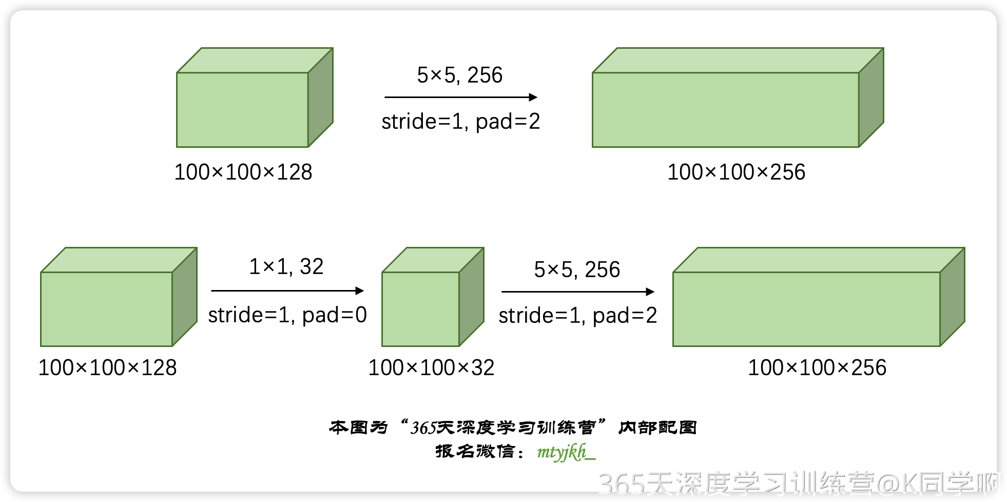
直接使用 5×5 卷积
- 输入:100 × 100 × 128
- 卷积核:5 × 5,数量 256
- 计算量: 5 × 5 × 128 × 100 × 100 × 256 ≈ 81.9 × 10 8 5 \times 5 \times 128 \times 100 \times 100 \times 256 \approx 81.9 \times 10^8 5×5×128×100×100×256≈81.9×10⁸
-
1×1 卷积降维后再进行 5×5 卷积
- 第一步:1×1 卷积降维
- 卷积核:1 × 1,数量 32
- 计算量: 1 × 1 × 128 × 100 × 100 × 32 = 4.096 × 10 7 1 \times 1 \times 128 \times 100 \times 100 \times 32 = 4.096 \times 10^7 1×1×128×100×100×32=4.096×10⁷
- 第二步:基于降维结果做 5×5 卷积
- 卷积核:5 × 5,数量 256
- 计算量: 5 × 5 × 32 × 100 × 100 × 256 = 20.48 × 10 8 5 \times 5 \times 32 \times 100 \times 100 \times 256 = 20.48 \times 10^8 5×5×32×100×100×256=20.48×10⁸
- 总计:计算量 ≈ 20.9 × 10 8 \approx 20.9 \times 10^8 ≈20.9×10⁸
- 结论:引入 1×1 卷积后,计算量下降了近 75%,极大地提升了计算效率。
- 第一步:1×1 卷积降维
-
-
-
卷积层的并行结构与 1×1 卷积核的作用
-
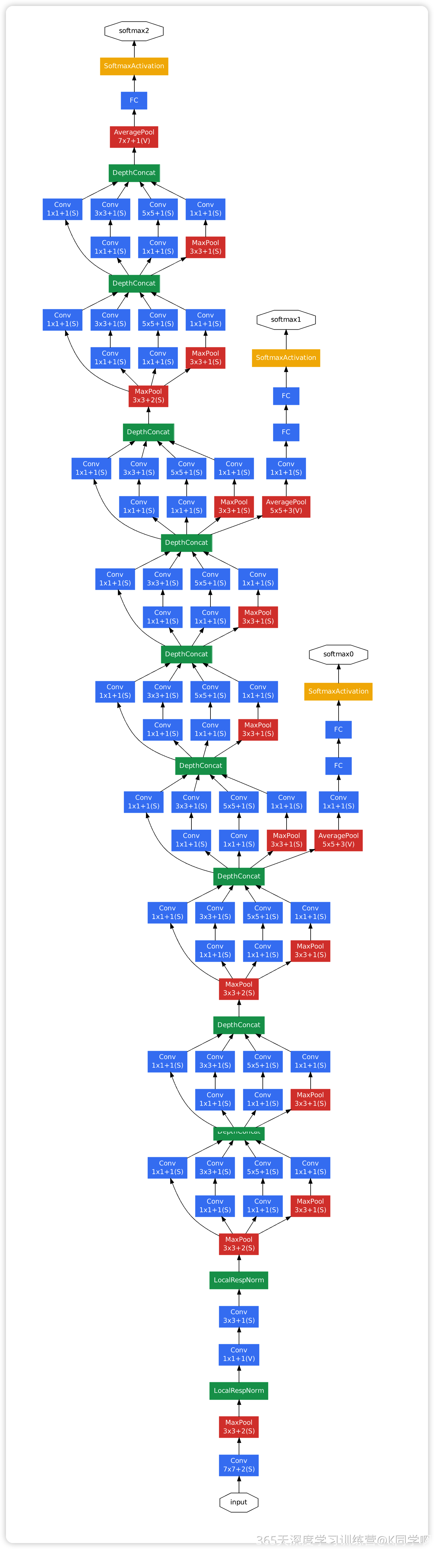
并行结构(Inception 模块):
- 传统网络是串行的单一尺寸卷积核,而 Inception 模块在同一层同时使用 1×1、3×3、5×5 卷积和最大池化。
- 因此并行可以在同一层提取多尺度的特征,大卷积核看全局轮廓,小卷积核看局部细节,最后通过
DepthConcat拼接融合。
-
1×1 卷积核的核心作用:
- 降维减负:在 3×3 或 5×5 卷积前,先用少量的 1×1 卷积核对输入通道进行压缩,大幅降低后续计算量。
-
代码实现
设置gpu
python
import torch
import torch.nn as nn
from torchvision import transforms, datasets
from PIL import Image
import matplotlib.pyplot as plt
import os,PIL,pathlib,warnings
warnings.filterwarnings("ignore") #忽略警告信息

device = torch.device("cuda" if torch.cuda.is_available() else "cpu")
device
数据导入
python
# 数据导入
data_dir = "../../datasets/MonkeyPox/"

train_transforms = transforms.Compose([
    transforms.Resize([224, 224]), # 将输入图片resize成统一尺寸
    transforms.ToTensor(), # 将图像转换为tensor,并归一化到[0,1]之间
    transforms.Normalize( # 转换为标准正太分布(高斯分布)
        mean=[0.485, 0.456, 0.406],
        std =[0.229, 0.224, 0.225])
])

total_data = datasets.ImageFolder(data_dir, transform = train_transforms)
total_data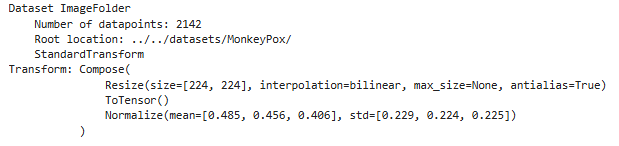
标签打印与数据集划分
python
total_data.class_to_idx
python
# 划分训练集和测试集(8:2)
total_size = len(total_data)
train_size = int(0.8 * total_size)
test_size = total_size - train_size
train_dataset, test_dataset = torch.utils.data.random_split(total_data, [train_size, test_size])
train_dataset, test_dataset
构建数据加载器 (DataLoader)
python
# 创建训练数据加载器:每次从训练集中加载 batch_size=32 个样本,并打乱顺序(shuffle=True)
train_loader = torch.utils.data.DataLoader(train_dataset,
                                           batch_size=32,
                                           shuffle=True)
# 创建测试数据加载器:每次从测试集中加载 batch_size=4 个样本,不打乱顺序(默认 shuffle=False)
test_loader = torch.utils.data.DataLoader(test_dataset,
                                          batch_size=32)
python
# 打印一个 batch 的数据形状以验证
for X, y in test_loader:
    print(f"输入张量形状 [Batch, Channel, Height, Width]: {X.shape}")
    print(f"标签形状: {y.shape}, 数据类型: {y.dtype}")
    break
构建 GoogLeNet (Inception v1)
python
import torch
import torch.nn as nn
import torch.nn.functional as F

class BasicConv2d(nn.Module):
    """基础卷积模块:Conv2d + ReLU"""
    def __init__(self, in_channels, out_channels, **kwargs):
        super(BasicConv2d, self).__init__()
        self.conv = nn.Conv2d(in_channels, out_channels, bias=False, **kwargs)
        self.relu = nn.ReLU(inplace=True)

    def forward(self, x):
        x = self.conv(x)
        x = self.relu(x)
        return x

class Inception(nn.Module):
    """Inception 模块 (对应图中的 4 个分支最后 DepthConcat 的结构)"""
    def __init__(self, in_channels, ch1x1, ch3x3red, ch3x3, ch5x5red, ch5x5, pool_proj):
        super(Inception, self).__init__()

        # 分支 1: 1x1 卷积
        self.branch1 = BasicConv2d(in_channels, ch1x1, kernel_size=1)

        # 分支 2: 1x1 卷积降维 -> 3x3 卷积
        self.branch2 = nn.Sequential(
            BasicConv2d(in_channels, ch3x3red, kernel_size=1),
            BasicConv2d(ch3x3red, ch3x3, kernel_size=3, padding=1) # 图中标注 (S) Same padding
        )

        # 分支 3: 1x1 卷积降维 -> 5x5 卷积
        self.branch3 = nn.Sequential(
            BasicConv2d(in_channels, ch5x5red, kernel_size=1),
            BasicConv2d(ch5x5red, ch5x5, kernel_size=5, padding=2) # 图中标注 (S) Same padding
        )

        # 分支 4: 3x3 最大池化 -> 1x1 卷积投影
        self.branch4 = nn.Sequential(
            nn.MaxPool2d(kernel_size=3, stride=1, padding=1),
            BasicConv2d(in_channels, pool_proj, kernel_size=1)
        )

    def forward(self, x):
        branch1 = self.branch1(x)
        branch2 = self.branch2(x)
        branch3 = self.branch3(x)
        branch4 = self.branch4(x)
        # 对应图中的 DepthConcat (在通道维度上拼接)
        return torch.cat([branch1, branch2, branch3, branch4], 1)

class InceptionAux(nn.Module):
    """对应图中的 softmax0 和 softmax1 分支"""
    def __init__(self, in_channels, num_classes):
        super(InceptionAux, self).__init__()
        # 图中标注: AveragePool 5x5+3(V)
        self.avgpool = nn.AvgPool2d(kernel_size=5, stride=3)
        # 图中标注: Conv 1x1+1(S)
        self.conv = BasicConv2d(in_channels, 128, kernel_size=1)
        # 两个全连接层 FC -> FC
        self.fc1 = nn.Linear(128 * 4 * 4, 1024)
        self.fc2 = nn.Linear(1024, num_classes)
        self.dropout = nn.Dropout(0.7)

    def forward(self, x):
        x = self.avgpool(x)
        x = self.conv(x)
        x = torch.flatten(x, 1)
        x = F.relu(self.fc1(x), inplace=True)
        x = self.dropout(x)
        x = self.fc2(x)
        return x

class GoogleNet(nn.Module):
    """主网络结构"""
    def __init__(self, num_classes=1000, aux_logits=True):
        super(GoogleNet, self).__init__()
        self.aux_logits = aux_logits

        # 输入及初始卷积池化部分
        # Conv 7x7+2(S)
        self.conv1 = BasicConv2d(3, 64, kernel_size=7, stride=2, padding=3)
        # MaxPool 3x3+2(S)
        self.maxpool1 = nn.MaxPool2d(3, stride=2, ceil_mode=True)
        # LocalRespNorm
        self.lrn1 = nn.LocalResponseNorm(5)

        # Conv 1x1+1(V)
        self.conv2 = BasicConv2d(64, 64, kernel_size=1)
        # Conv 3x3+1(S)
        self.conv3 = BasicConv2d(64, 192, kernel_size=3, padding=1)
        # LocalRespNorm
        self.lrn2 = nn.LocalResponseNorm(5)
        # MaxPool 3x3+2(S)
        self.maxpool2 = nn.MaxPool2d(3, stride=2, ceil_mode=True)

        # Inception 模块组 1
        self.inception3a = Inception(192, 64, 96, 128, 16, 32, 32)
        self.inception3b = Inception(256, 128, 128, 192, 32, 96, 64)
        self.maxpool3 = nn.MaxPool2d(3, stride=2, ceil_mode=True)

        # Inception 模块组 2
        self.inception4a = Inception(480, 192, 96, 208, 16, 48, 64)

        # (图中的 softmax0) 挂载在 Inception 4a 之后
        if self.aux_logits:
            self.aux1 = InceptionAux(512, num_classes)

        self.inception4b = Inception(512, 160, 112, 224, 24, 64, 64)
        self.inception4c = Inception(512, 128, 128, 256, 24, 64, 64)
        self.inception4d = Inception(512, 112, 144, 288, 32, 64, 64)

        # (图中的 softmax1) 挂载在 Inception 4d 之后
        if self.aux_logits:
            self.aux2 = InceptionAux(528, num_classes)

        self.inception4e = Inception(528, 256, 160, 320, 32, 128, 128)
        self.maxpool4 = nn.MaxPool2d(2, stride=2, ceil_mode=True)

        # Inception 模块组 3 及最终输出
        self.inception5a = Inception(832, 256, 160, 320, 32, 128, 128)
        self.inception5b = Inception(832, 384, 192, 384, 48, 128, 128)

        # AveragePool 7x7+1(V)
        self.avgpool = nn.AdaptiveAvgPool2d((1, 1))
        self.dropout = nn.Dropout(0.4)
        # 最后的 FC -> SoftmaxActivation -> softmax2
        self.fc = nn.Linear(1024, num_classes)

    def forward(self, x):
        # 底部特征提取
        x = self.conv1(x)
        x = self.maxpool1(x)
        x = self.lrn1(x)
        x = self.conv2(x)
        x = self.conv3(x)
        x = self.lrn2(x)
        x = self.maxpool2(x)

        # Inception 组 1
        x = self.inception3a(x)
        x = self.inception3b(x)
        x = self.maxpool3(x)

        # Inception 组 2
        x = self.inception4a(x)

        # 输出分支 1: aux1
        aux1 = None
        if self.aux_logits and self.training:
            aux1 = self.aux1(x)

        x = self.inception4b(x)
        x = self.inception4c(x)
        x = self.inception4d(x)

        # 输出分支 2: aux2
        aux2 = None
        if self.aux_logits and self.training:
            aux2 = self.aux2(x)

        x = self.inception4e(x)
        x = self.maxpool4(x)

        # Inception 组 3
        x = self.inception5a(x)
        x = self.inception5b(x)

        # 最终分类器
        x = self.avgpool(x)
        x = torch.flatten(x, 1)
        x = self.dropout(x)
        x = self.fc(x)

        # 在训练时返回主分类器和两个分支的结果,测试时只返回主分类器结果
        if self.training and self.aux_logits:
            return x, aux2, aux1
        return x

# 实例化 GoogleNet 模型
model = GoogleNet().to(device)

# 查看模型结构
import torchsummary as summary
summary.summary(model, (3, 224, 224))
训练和测试函数
python
# 训练循环
def train(dataloader, model, loss_fn, optimizer):
    size = len(dataloader.dataset) # 训练集的大小
    num_batches = len(dataloader) # 批次数目(size/batch_size,向上取整)

    train_loss, train_acc = 0, 0 # 初始化训练损失和正确率

    for X, y in dataloader: # 获取图片及其标签
        X, y = X.to(device), y.to(device)

        # 因为是 GoogLeNet 的训练模式,网络会吐出 3 个结果,我们要拿 3 个变量接住它
        pred, aux2, aux1 = model(X)

        # 分别计算三个结果的误差,然后按 1 : 0.3 : 0.3 的比例加起来
        loss_main = loss_fn(pred, y)
        loss_aux2 = loss_fn(aux2, y)
        loss_aux1 = loss_fn(aux1, y)
        loss = loss_main + 0.3 * loss_aux2 + 0.3 * loss_aux1

        # 反向传播
        optimizer.zero_grad() # grad属性归零
        loss.backward() # 反向传播
        optimizer.step() # 每一步自动更新

        # 记录acc和loss。注意算正确率的时候,只看主输出(pred)到底猜得准不准,不管分支的
        train_acc += (pred.argmax(1) == y).type(torch.float).sum().item()
        train_loss += loss.item()

    train_acc /= size # 计算训练集整体正确率
    train_loss /= num_batches # 计算训练集平均损失

    return train_acc, train_loss
python
# 测试函数
def test(dataloader, model, loss_fn):
    size = len(dataloader.dataset) # 测试集的大小
    num_batches = len(dataloader)  # 批次数目(size/batch_size,向上取整)
    test_loss, test_acc = 0, 0

    # 当不进行训练时,停止梯度更新,节省计算内存消耗
    with torch.no_grad():
        for imgs, target in dataloader:
            imgs, target = imgs.to(device), target.to(device)

            # 计算loss
            target_pred = model(imgs)
            loss = loss_fn(target_pred, target)

            test_loss += loss.item()
            test_acc += (target_pred.argmax(1) == target).type(torch.float).sum().item()

    test_acc /= size
    test_loss /= num_batches

    return test_acc, test_loss
正式训练
python
# 训练
import copy
import torch
import torch.nn as nn
import torch.optim as optim

# 初始化优化器与损失函数
optimizer = optim.AdamW(model.parameters(), lr=1e-4)
loss_fn = nn.CrossEntropyLoss()  # 创建损失函数

epochs = 100  # 训练轮数

# 每 15 轮把学习率砍一半
scheduler = optim.lr_scheduler.StepLR(optimizer, step_size=15, gamma=0.5)
# 初始化指标记录列表
train_loss = []
train_acc = []
test_loss = []
test_acc = []

best_acc = 0  # 设置最佳准确率,作为保存最佳模型的指标

for epoch in range(epochs):

    # 训练阶段
    model.train()  # 开启训练模式(启用 Dropout、BatchNorm 等层的训练行为)
    epoch_train_acc, epoch_train_loss = train(train_loader, model, loss_fn, optimizer)

    # 测试阶段
    model.eval()  # 开启评估模式(禁用 Dropout、固定 BatchNorm 等层的参数)
    epoch_test_acc, epoch_test_loss = test(test_loader, model, loss_fn)

    scheduler.step()

    # 保存最佳模型
    if epoch_test_acc > best_acc:
        best_acc = epoch_test_acc
        best_model = copy.deepcopy(model)  # 深拷贝当前最佳模型

    # 记录训练/测试指标
    train_acc.append(epoch_train_acc)
    train_loss.append(epoch_train_loss)
    test_acc.append(epoch_test_acc)
    test_loss.append(epoch_test_loss)

    # 获取当前学习率
    lr = optimizer.state_dict()['param_groups'][0]['lr']

    # 打印当前轮次的指标
    template = ('第 {:2d} 轮,训练准确率:{:.1f}%,训练损失:{:.3f},测试准确率:{:.1f}%,测试损失:{:.3f},学习率:{:.2E}')
    print(template.format(epoch + 1,
                          epoch_train_acc * 100,
                          epoch_train_loss,
                          epoch_test_acc * 100,
                          epoch_test_loss,
                          lr))

# 保存最佳模型到文件
PATH = './best_model.pth'  # 保存的参数文件名
torch.save(best_model.state_dict(), PATH)  # 保存模型的参数状态字典

print('完成')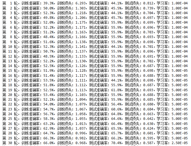
可视化训练结果
python
# 结果可视化
import matplotlib.pyplot as plt
# 隐藏警告
import warnings
warnings.filterwarnings("ignore")  # 忽略警告信息

# 配置 Matplotlib 显示(解决中文/负号显示问题)
plt.rcParams['font.sans-serif'] = ['SimHei'] # 正常显示中文标签
plt.rcParams['axes.unicode_minus'] = False # 正常显示负号
plt.rcParams['figure.dpi'] = 100 # 设置图像分辨率为 100

from datetime import datetime
current_time = datetime.now() # 获取当前时间

epochs_range = range(epochs)

# 创建画布并绘制子图
plt.figure(figsize=(12, 3))

# 子图 1:准确率曲线
plt.subplot(1, 2, 1)
plt.plot(epochs_range, train_acc, label='训练准确率')
plt.plot(epochs_range, test_acc, label='测试准确率')
plt.legend(loc='lower right')
plt.title('训练与验证准确率')
plt.xlabel(f'训练轮次(生成时间:{current_time.strftime("%Y-%m-%d %H:%M:%S")})')  # 横轴标注当前时间

# 子图 2:损失曲线
plt.subplot(1, 2, 2)
plt.plot(epochs_range, train_loss, label='训练损失')
plt.plot(epochs_range, test_loss, label='测试损失')
plt.legend(loc='upper right')
plt.title('训练与验证损失')

plt.show()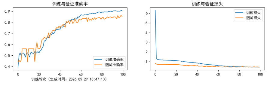
预测
python
from PIL import Image

classes = list(total_data.class_to_idx)

def predict_one_image(image_path, model, transform, classes):

    test_img = Image.open(image_path).convert('RGB')
    # plt.imshow(test_img)  # 展示预测的图片

    test_img = transform(test_img)
    img = test_img.to(device).unsqueeze(0)

    model.eval()
    output = model(img)

    _,pred = torch.max(output,1)
    pred_class = classes[pred]
    print(f'预测结果是:{pred_class}')
python
# 预测训练集中的某张照片
predict_one_image(image_path='../../datasets/MonkeyPox/MonkeyPox/M01_01_00.jpg',
                  model=model,
                  transform=train_transforms,
                  classes=classes)
python
predict_one_image(image_path='../../datasets/MonkeyPox/Others/NM01_01_00.jpg',
                  model=model,
                  transform=train_transforms,
                  classes=classes)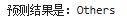
总结
这周复现了 GoogleNet(Inception v1),除了对inceptionv1结构有了了解,还对震荡有了新的认识。
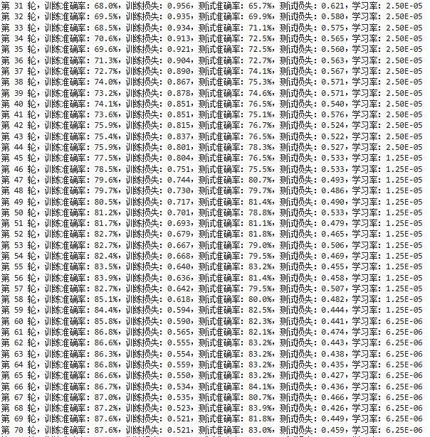
第 26~55 轮是震荡最猛的阶段。主要的猜测原因如下:
- 学习率还比较大(1e-4 ~ 2.5e-5),模型每次更新参数的幅度不低,导致它的"决策边界"一直在晃。同一张图,上一轮在边界右边(猜对),这一轮参数一更新,边界移了,这张图就跑到左边了(猜错)。等再更新一轮,又回来了。
- 多个分支在"打架":Inception 结构里四个分支(1x1、3x3、5x5、池化)并行工作。这个阶段各个侦探的权重还在激烈争夺主导权------这轮 3x3 侦探权重高一点,下轮 5x5 侦探权重高一点,最终拼出来的结果就忽上忽下。
- 分支的分类器在起作用, Loss 是主输出 + 0.3×分支1 + 0.3×分支2。这两个分支分类器从半路拉出来做判断,它们的梯度也会影响前面的层。
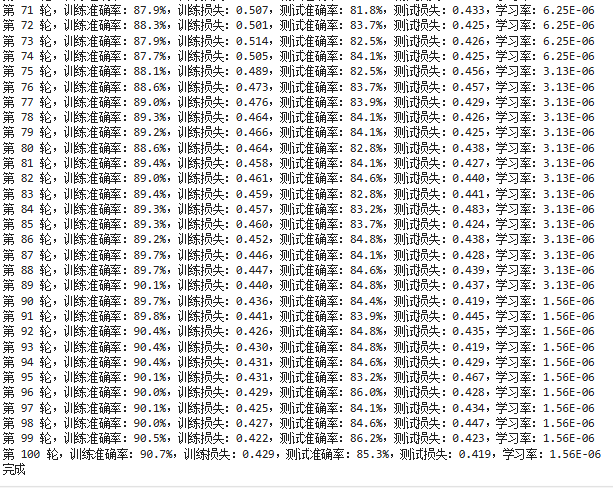
而第 56~100 轮的震荡猜测是过拟合造成的,测试准确率在 82%~86% 之间反复横跳,就是不继续涨了。与此同时训练准确率稳步从 85% 爬到 90%,这很像是过拟合。模型已经把训练集背下来了(90.7%),但测试集里有一些它没见过的新花样(不同的光照、角度、背景等)。每次测试,只要这批图里包含几张它不擅长的那类图片,准确率就掉到 82%;如果这批碰巧都是擅长的,就跳到 86%。